Configuración del controlador.
El PID es uno de los controladores más ampliamente utilizados en los esquemas de compensación siguientes, algunas de las cuáles se ilustran en la Figura 10-2:
- Compensación en serie (cascada),
- Compensación mediante realimentación,
- Compensación mediante realimentación de estado,
- Compensación en serie-realimentada,
- Compensación prealimentada,


En general, la dinámica de un proceso lineal controlado puede representarse mediante el diagrama de la Figura 10-1.


El objetivo de diseño es que las variables controladas, representadas por el vector de salida y(t), se comporten de cierta forma deseada. El problema esencialmente involucra el determinar la señal de control u(t) dentro de un intervalo prescrito para que todas las especificaciones de diseño sean satisfechas (ver Estabilidad de un sistema de control, Respuesta transitoria, Error en estado estable).
El controlador PID aplica una señal al proceso de control mostrado en la Figura 10-1, que es una combinación proporcional, integral y derivada de las señal de actuación e(t). Debido a que estos componentes de la señal se pueden realizar y visualizar fácilmente en el dominio del tiempo, los controladores PID se diseñan comúnmente empleando métodos en el dominio del tiempo.
Después de que el diseñador ha seleccionado una configuración para el controlador, debe escoger además el tipo de controlador. En general, mientras más complejo el controlador, más costoso, menos confiable y más difícil de diseñar. Por ende, en la práctica se selecciona el tipo de controlador más simple que permita cumplir con las especificaciones de diseño, lo que involucra experiencia, intuición, arte y ciencia.
Las componentes integral y derivativo de un controlador PID tienen una implicación individual en el desempeño, y sus aplicaciones requieren un entendimiento de las bases de estos elementos. Por ello, se consideran por separado, iniciando con la porción PD.
Diseño con el controlador PD

La Figura 10-3 muestra el diagrama de bloques de un sistema de control realimentado que deliberadamente tiene una planta prototipo de segundo orden con la siguiente función de transferencia Gp(s):

El controlador en serie es del tipo proporcional-derivativo (PD) con la función de transferencia:

Por lo tanto, la señal de control U(s) aplicada a la planta es:

en donde Kp y Kd son las constantes proporcional y derivativa respectivamente, mientras E(s) es la señal de error. La realización del controlador PD mediante circuitos electrónicos se muestra en la Figura 10-4:


La función de transferencia del circuito de la Figura 10-4 es:

Al comparar con la Figura 10-3:

La función de transferencia directa del compensador mostrado en la Figura 10-3 es:

lo cual muestra que el control PD equivale a añadir un cero simple en s=-Kp/Kd a la función de transferencia directa. El efecto de control PD sobre la respuesta transitoria de un sistema de control se puede investigar al referirse a la respuesta en tiempo del sistema como se muestra en la Figura 10-5:

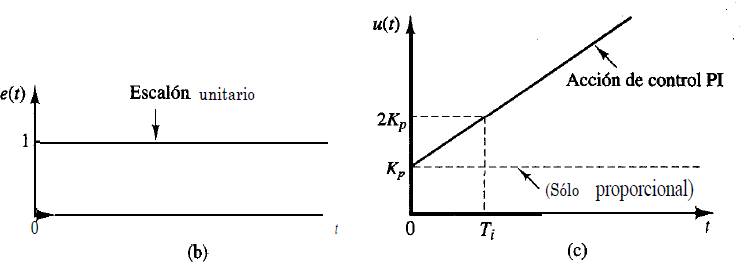
Se supone que la respuesta al escalón unitario de un sistema estable con el control proporcional es solamente como la que se presenta en la Figura 10-5(a). Se observa un sobrepaso máximo relativamente grande y un poco oscilatorio. La señal de error e(t) correspondiente, que es la diferencia entre la entrada r(t) escalón unitario y la salida y(t), y la derivada de dicho error en el tiempo, se muestran en las Figuras (b) y (c) respectivamente.
Durante el intervalo 0<t<t1, la señal de error es positiva, el sobrepaso es grande y se observa gran oscilación en la salida debido a la falta de amortiguamiento en este período. Durante el intervalo t1<t<t2, la señal de error es negativa, la salida se invierte y tiene un sobrepaso negativo. Este comportamiento se alterna sucesivamente hasta que la amplitud del error se reduce con cada oscilación, y la salida se establece eventualmente en su valor final. Se observa que el controlador PD puede añadir amortiguamiento a un sistema y reduce el sobrepaso máximo, pero no afecta el estado estable directamente.
Ejemplo.
Para apreciar mejor el efecto del controlador PD, veamos el siguiente ejemplo. Supongamos que tenemos el sistema de la Figura 7-23.

La función de transferencia directa G(s) de este sistema viene dada por la siguiente expresión: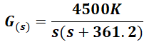
Donde K es la constante del preamplificador.
Las especificaciones de diseño para este sistema son las siguientes:
 Donde:
- ess: Error en estado estable debido a una entrada de rampa unitaria
- Mp: Sobrepaso máximo
- Tr: Tiempo de levantamiento
- Ts: Tiempo de asentamiento
- Selección del valor de K
Lo primero que vamos a hacer es hallar K para cumplir con el primer requerimiento de diseño, error en estado estable ess debido a una entrada rampa:

(Para repasar el concepto de error en estado estable ver Error en estado estable de un sistema de control)
1.a Hallar la constante de velocidad Kv porque es la relacionada a una entrada rampa:

1.b Hallar ess en función de K:

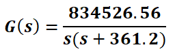
1.c Hallar K para ess=0.000433:

Con este valor de K, la función de transferencia directa G(s) es:
2. Cálculo de sobrepaso
Veamos ahora como queda el sobrepaso para el valor de K obtenido.
(Para un repaso del concepto de sobrepaso y la respuesta transitoria ver Respuesta Transitoria de un Sistema de Control)
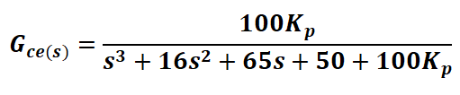
2.a La función de transferencia de lazo cerrado Gce(s) es:

2.b Hallamos a partir de aquí el factor de amortiguamiento relativo ζ y la frecuencia natural del sistema ωn.

2.c Con estos valores, hallamos el sobrepaso máximo Mp:

En porcentaje:

Este valor supera la exigencia de la especificación, por lo que se considera insertar un controlador PD en la trayectoria directa del sistema con el fin de mejorar el amortiguamiento y ajustar el sobrepaso máximo a la especificación de diseño exigida, manteniendo sin embargo el error en estado estable en 0.000433.
3. Diseño en el dominio del tiempo del controlador PD
Añadiendo el controlador Gc(s) de la Figura 10-3 a la trayectoria directa del sistema aeronáutico, y asignando K=185.4503, la función de transferencia directa G(s) del sistema de control de posición de la aeronave es:

Mientras, la función de transferencia a lazo cerrado Gce(s) es:

Esta última ecuación muestra los efectos del controlador PD sobre la función de transferencia de lazo cerrado del sistema al cual se aplica:
- Añadir un cero en s=-Kp/Kd
- Incrementar el “término asociado al amortiguamiento”, el cual es el coeficiente de s en el denominador de Gce(s). Es decir, de 361.2 hasta 361.2 + 834526.56Kd
3.a Selección de Kp
Para asegurarnos de que se mantenga el error en estado estable para una entrada rampa de acuerdo con las especificaciones, evaluamos dicho error y seleccionamos un valor para Kp:

Al elegir Kp igual a uno, mantenemos el mismo valor para Kv que se tenía antes de añadir el controlador. Es decir, mantenemos el valor del error en estado estable para entrada rampa tal como lo exige la especificación de diseño. Entonces: 3.b Selección de Kd
De acuerdo con la ecuación de sobrepaso máximo:

El sobrepaso máximo depende del factor de amortiguamiento relativo ζ. La ecuación característica del sistema es:

Donde:

Deducimos la expresión para el factor de amortiguamiento relativo ζ:

Este resultado muestra claramente el efecto positivo de Kd sobre el amortiguamiento. Sin embargo, se debe resaltar el hecho de que la función de transferencia directa G(s) ya no representa un sistema prototipo de segundo orden, por lo que la respuesta transitoria también se verá afectada por el cero en s=-Kp/Kd.
Aplicaremos ahora el método del lugar geométrico de la raíces a la ecuación característica para examinar el efecto de variar Kd, mientras se mantiene constante el valor de Kp=1.
(Para un repaso ver El lugar geométrico de las raíces de un sistema de control – 1era. parte. / El lugar geométrico de las raíces con Matlab)
Si deseamos obtener un Mp=5% tal y como se pide en las especificaciones de diseño, eso significa obtener un factor de amortiguamiento relativo igual a lo siguiente:

La ecuación característica del sistema y su forma 1+G(s)H(s) son:
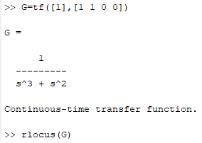
Utilizando el siguiente comando en Matlab obtenemos el lugar geométrico de las raíces para G(s)H(s):
>> s=tf(‘s’)
>> sys=(834526.56*s)/(s^2+361.2*s+834526.56)
>> rlocus(sys)

La gráfica siguiente muestra como mejora el factor de amortiguamiento relativo ζ a medida que aumenta la ganancia Kd:

Mientras, en la gráfica siguiente se muestra que para lograr un factor de amortiguamiento relativo ζ=0.69 o mejor que ese, lo cual significa un sobrepaso menor de 5% como se especifica, es necesario tener una ganancia mínima Kd= 0.00108:

Sin embargo, antes de seleccionar un valor definitivo para Kd debemos observar el cumplimiento de los otros requerimientos de diseño.
3.c Evaluación de Tr y Ts según Kd y Kp calculados.
Analizamos a continuación el valor del tiempo de levantamiento Tr para el valor de ζ=0.69 , Kd= 0.00108 y Kp= 1, utilizando la función de transferencia a lazo cerrado del sistema Gce(s) y el gráfico de respuesta a la entrada escalón generado por el siguiente comando en Matlab:
>> s=tf(‘s’)
>>sys=(834526.56*(1+0.00108*s))/(s^2+(361.2+834526.56*0.00108)*s+834526.56)
sys = (901.3 s + 8.345e05) / (s^2 + 1262 s + 8.345e05)
> step(sys)

Utilizando la gráfica para la salida C(t) del sistema a una entrada escalón para un valor determinado del factor de amortiguamiento relativo (ζ=0.69). Para hallar Tr, restamos los tiempos para los cuáles C(t)=0.9 y C(t)=0.1:

La gráfica anterior nos permite determinar el valor de Tr para un valor de ζ=0.69 de la siguiente manera:

Podemos ver que este valor cumple con el requerimiento de que Tr≤0.005 s. Veamos ahora que pasa con Ts. Utilizando el criterio del 2% podemos calcular Ts mediante la siguiente fórmula:
Así vemos que el factor de amortiguamiento ζ=0.69 genera un Ts que no cumple con la condición de un Ts menor o igual a 0.005 s. Sin embargo, aumentando Kd mejoramos ζ logrando satisfacer dicha condición. Para ser más específicos, despejamos ζ a partir del valor máximo aceptado para Ts:

Utilizamos nuevamente el lugar geométrico de las raíces para determinar el valor de Kd que se corresponde con el de ζ=0.8757:

Si el valor de Kd=0.00148 y mantenemos el valor de Kp=1, la función de transferencia directa es:
Mientras, la función de transferencia a lazo cerrado del sistema en estudio es la siguiente:
Para esta función de transferencia revisamos los valores de sobrepaso Mp y tiempo de levantamiento Tr para asegurarnos que cumplen con las especificaciones de diseño:


Por tanto, el valor de Kd debe tener un valor mínimo de:

Y nuestro controlador PD puede tener entonces la siguiente función de transferencia:

ANTERIOR: PID – Efecto de las acciones de control Proporcional, Integral y Derivativo
Escrito por: Larry Francis Obando – Technical Specialist – Educational Content Writer.
Mentoring Académico / Empresarial / Emprendedores
Copywriting, Content Marketing, Tesis, Monografías, Paper Académicos, White Papers (Español – Inglés)
Escuela de Ingeniería Eléctrica de la Universidad Central de Venezuela, Caracas.
Escuela de Ingeniería Electrónica de la Universidad Simón Bolívar, Valle de Sartenejas.
Escuela de Turismo de la Universidad Simón Bolívar, Núcleo Litoral.
Contact: Caracas, Quito, Guayaquil, Cuenca – Telf. 00593998524011
WhatsApp: +593981478463
+593998524011
email: dademuchconnection@gmail.com
| Atención:
Si lo que Usted necesita es resolver con urgencia un problema de “Sistema Masa-Resorte-Amortiguador” (encontrar la salida X(t), gráficas en Matlab del sistema de 2do Orden y parámetros relevantes, etc.), o un problema de “Sistema de Control Electromecánico” que involucra motores, engranajes, amplificadores diferenciales, etc…para entregar a su profesor en dos o tres días, o con mayor urgencia…o simplemente necesita un asesor para resolver el problema y estudiar para el próximo examen…envíeme el problema…Yo le resolveré problemas de Sistemas de Control, le entrego la respuesta en digital y le brindo una video-conferencia para explicarle la solución…incluye además simulación en Matlab. |
Relacionado:
Respuesta Transitoria de un Sistema de Control
Estabilidad de un sistema de control
Simulación de Respuesta Transitoria con Matlab – Introducción


 Reshaping:
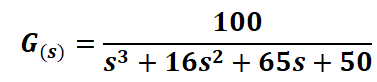 If we add a proportional controller with a gain Kp, the direct transfer function G(s) is:
 Th closed-loop transfer function Gce(s) is:
 The characteristic equation is:
 The characteristic equation in its form 1+G(s)H(s) is:


 Donde:
 This means an infinite error for a parabolic input:
 To improve the steady-state error we incorporate a PI controller in the direct path of the system, which will now have the following transfer function:
 By increasing the typology of the system from type 1 to type 2 we immediately improve the steady-state error. Now, the ess due to the parabolic input will be a constant:
 That is to say:


 With this result, the direct transfer function G(s):
 It would be simplified as: