Bode Diagram, Control System Analysis, Transfer function

Obtaining Transfer Function from Bode Diagram

Bode plots are a convenient presentation of the frequency response data for
the purpose of estimating the transfer function. These plots allow parts of the
transfer function to be determined and extracted, leading the way to further
refinements to find the remaining parts of the transfer function.

Although experience and intuition are invaluable in the process, the following steps are still offered as a guideline:

1. Look at the Bode magnitude and phase plots and estimate the pole-zero configuration of the system. Look at the initial slope on the magnitude plot to determine system type. Look at phase excursions to get an idea of the difference between the number of poles and the number of zeros.
2. See if portions of the magnitude and phase curves represent obvious first- or second-order pole or zero frequency response plots.
3. See if there is any telltale peaking or depressions in the magnitude response plot that indicate an underdamped second-order pole or zero, respectively.
4. If any pole or zero responses can be identified, overlay appropriate ±20 or ±40 dB/decade lines on the magnitude curve or ±45°/decade lines on the phase curve and estimate the break frequencies.For second-order poles or zeros, estimate the damping ratio and natural frequency from the standard curves.
5. Form a transfer function of unity gain using the poles and zeros found. Obtain the frequency response of this transfer function and subtract this response from the previous frequency response (Franklin, 1991). You now have a frequency response of reduced complexity from which to begin the process again to extract more of the system’s poles and zeros. A computer program such as MATLAB is of invaluable help for this step.

Example

Find the transfer function of the subsystem whose Bode plots are shown in Figure 1:

null

Figure 1

Let us first extract the underdamped poles that we suspect, based on the peaking in the magnitude curve.We estimate the natural frequency to be near the peak frequency, or approximately 5 rad/s. From Figure 1, we see a peak of about 6.5 dB, which translates into a damping ratio of about ζ=0,24. The unity gain second-order function is thus:

null

The frequency response plot of this function is made and subtracted from the previous
Bode plots to yield the response in Figure 2:
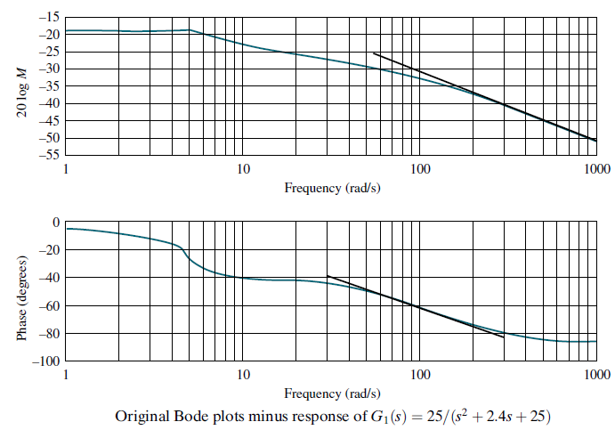
null

Figure 2

Overlaying a -20 dB/decade line on the magnitude response and a -45°/decade line on the phase response, we detect a final pole. From the phase response, we estimate the break frequency at 90 rad/s. Subtracting the response of G2(s)=90/(s+90) from the previous response yields the response in Figure 3.

null

Figure 3

Figure 3 has a magnitude and phase curve similar to that generated by a lag function. We draw a -20 dB/decade line and fit it to the curves. The break frequencies are read from the figure as 9 and 30 rad/s. A unity gain transfer function containing a pole at -9 and a zero at -30 is G3(s)=0.3(s+30)/(s+9). Upon subtraction of G1(s)G2(s)G3(s), we find the magnitude frequency response flat ±1 dB and the phase response flat at -3± 5°. We thus conclude that we are finished extracting dynamic transfer functions as:

null

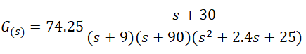
It is interesting to note that the original curve was obtained from the function:

null

Sources:

  1. Modern_Control_Engineering, Ogata 4t
  2. Control Systems Engineering, Nise
  3. Sistemas de Control Automatico, Kuo

Literature review by:

Prof. Larry Francis Obando – Technical Specialist – Educational Content Writer

Resolving problems!!

WhatsApp:  +34633129287  Immediate attention!!

Twitter: @dademuch

Copywriting, Content Marketing, Tesis, Monografías, Paper Académicos, White Papers (Español – Inglés)

Escuela de Ingeniería Electrónica de la Universidad Simón Bolívar, USB Valle de Sartenejas.

Escuela de Ingeniería Eléctrica de la Universidad Central de Venezuela, UCV CCs

Escuela de Turismo de la Universidad Simón Bolívar, Núcleo Litoral.

Contacto: España. +34633129287

Caracas, Quito, Guayaquil, Cuenca. 

WhatsApp:  +34633129287   +593998524011  

Twitter: @dademuch

FACEBOOK: DademuchConnection

email: dademuchconnection@gmail.com


Bode Diagram

The Bode Diagrams – Plotting of the frequency response of a control system.

The Bode Diagrams is the plotting of the frequency response of a system with separate magnitude and phase plots. The log-magnitude and phase frequency response curves as functions of log ω  are called Bode plots or Bode diagrams. Sketching Bode plots can be simplified because they can be approximated as a sequence of straight lines. Straight-line approximations simplify the evaluation of the magnitude and phase frequency response.

When plotting separate magnitude and phase plots, the magnitude curve can be plotted in decibels (dB) vs. log ω, where dB = 20 log M. Meanwhile, the phase curve is plotted as phase angle vs. log ω.

Example

Plot The Bode Diagram for the frequency response of the characterized by the system Transfer Function G(s):

null

null

Basic Factors of G(jω)H(jω)

The main advantage of using a logarithmic trace is the relative ease of plotting the frequency response curves. The basic factors that are frequent in an arbitrary transfer function G(jω)H(jω) are:

  1. The gain K
  2. Integral and derivative factors null,
  3. First order factors null,
  4. The quadratic factors null.

Once we become familiar with the logarithmic traces of these basic factors, it is possible to use them in order to construct a composite logarithmic trace for any form of G(jω)H(jω), plotting the curves for each factor and adding individual curves in graphical form, since adding the logarithms of the gains corresponds to multiplying them among themselves.

The process of obtaining the logarithmic trace is further simplified by asymptotic approximations for the curves of each factor.

The gain K. A number greater than the unit has a positive value in decibels, while a number smaller than the unit has a negative value.

The logarithmic magnitude curve for a constant gain K is a horizontal line whose magnitude is 20 log K decibels. The phase angle of the gain K is zero. The effect of varying the gain K in the transfer function is that the logarithmic magnitude curve of the transfer function is raised or lowered by the corresponding constant amount, but does not affect the phase curve.

Integral and derivative factorsnull(Poles and Zeros in the origin). The logarithmic magnitude of l/ in decibels is:

null

The phase angle of l/ is constant and equal to -90 °.

In Bode’s Diagram, the frequency ratios are expressed in terms of octaves or decades. An octave is a frequency band from ω1 to 2ω1, where ω1 is any frequency. A decade is a frequency band from ω1 to 10ω1, where, again, ω1 is any frequency. (On the logarithmic scale of the semi-logarithmic paper, any given frequency ratio is represented by the same horizontal distance. For example, the horizontal distance of ω=1  to ω=10 is equal to that of ω=3  to ω=30.

If the logarithmic magnitude of -20 log ω dB is plotted against ω on a logarithmic scale, a line is obtained. To draw this line, we need to locate a point (0 dB, ω= 1) on it. Given that:

null

The slope m of the line for l/ is:

null

The phase angle of the factor l/ is constant and equal to -90°.

Smilarly:null

The slope m of the line for is:null

The phase angle of the factor  is constant and equal to -90°.

The following figure shows frequency response curves for l/ and , respectively.

null

Note that both logarithmic quantities become equal to 0 dB at ω=1.

Therefore, if the transfer function contains the factor (l/)n or ()n, the logarithmic magnitude becomes, respectively, in:

nullOr well:

null

Therefore, the slopes of the logarithmic magnitude curves for the factors (l/)n and ()n are -20n dB/decade und 20n dB/decade, respectively.

The phase angle of (l/)n is equal to -90°n over the entire frequency range, while the phase angle of ()n is equal to 90°n over the entire frequency range. The magnitude curves will pass through the point (0 dBω= 1).

First order Factorsnull. The logarithmic magnitude of l/(1+jωT) in decibels is:

null

For low frequencies, such that ω<<1/T, the logarithmic magnitude is approximated by:

null

Therefore, the logarithmic magnitude curve for low frequencies in this factor is the constant 0 dB line. For high frequencies, such that:

null

The latter is an approximate expression for the high frequency range. At ω=1/T, the logarithmic magnitude is equal to 0 dB; at ω=10/T, the logarithmic magnitude is -20 dB. Therefore, the value of -20 log ωT dB decreases by 20 dB for all decades of ω. Thus, for ω>>1/T, the logarithmic magnitude curve is a straight line with a slope of -20dB/decade (or -6 dB/octave).

Our analysis shows that the logarithmic representation of the frequency response curve of the factor l/(1+jωT) is approximated by two asymptotes (straight lines), one of which is a straight line of 0 dB for the frequency range 0<ω<1/T and the other is a straight line with a slope of -20 dB/decade (or -6 dB/octave) for the frequency range 1/T<ω<∞. The frequency in which the two asymptotes meet is called the corner frequency or cutoff frequency. For the factor l/(1+jωT), the frequency ω=1/T is the corner frequency, since at that point both asymptotes have the same value.

null

An advantage of Bode Diagrams is that, for reciprocal factors, for example, the factor 1+jωT, the logarithmic magnitude and phase angle curves only need to change sign. Therefore, the slope of the high frequency asymptote of 1+jωT is 20 dB/decade, and the phase angle varies from 0° to 90° as the frequency ω increases from zero to infinity, as can be seen in the following figure:

null

Quadratic Factorsnull. Control systems usually have quadratic factors of the form:null

If ζ>1, this quadratic factor is expressed as a product of two first-order factors with real poles. If 0<ζ<1, this quadratic factor is the product of two complex conjugate factors.

The asymptotic frequency response curve for null is obtained as follows. Given that:

null

For low frequencies such that ω<<ωn, the logarithmic magnitude becomes:

null

Therefore, the low frequency asymptote is a horizontal line at 0 dB. For high frequencies such that ω>>ωn, the logarithmic magnitude becomes:

null

The equation for the high frequency asymptote is a line with a slope of -40dB/decade, given that:

null

The high frequency asymptote intersects the low frequency at ω=ωn, since at this frequency:

null

This frequency ωn is the corner frequency for the quadratic factor considered.

null

Sources:

  1. Modern_Control_Engineering, Ogata 4t
  2. Control Systems Engineering, Nise
  3. Sistemas de Control Automatico, Kuo

Literature review by:

Prof. Larry Francis Obando – Technical Specialist – Educational Content Writer

Se hacen trabajos, se resuelven ejercicios!!

WhatsApp:  +34633129287  Atención Inmediata!!

Twitter: @dademuch

Copywriting, Content Marketing, Tesis, Monografías, Paper Académicos, White Papers (Español – Inglés)

Escuela de Ingeniería Electrónica de la Universidad Simón Bolívar, USB Valle de Sartenejas.

Escuela de Ingeniería Eléctrica de la Universidad Central de Venezuela, UCV CCs

Escuela de Turismo de la Universidad Simón Bolívar, Núcleo Litoral.

Contacto: España. +34633129287

Contact: Caracas, Quito, Guayaquil, Jaén, Villafranca de Ordizia- Telf. +34633129287

WhatsApp:  +34633129287   +593998524011  

Twitter: @dademuch

FACEBOOK: DademuchConnection

email: dademuchconnection@gmail.com