Control System Analysis, Transfer function

Open loop and closed loop transfer function – examples

To understand the concept of Transfer Function in open loop, or on the contrary, closed loop, we use a block diagram of a closed loop system, Figure 1:
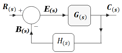
null

Figure 1

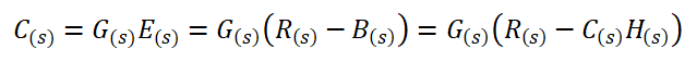
Where G (s) is the transfer function of the plant and H (s) is the transfer function of the sensor. The sensor generates a signal B (s) that is fed back to the summing point, where it is compared with the reference signal R (s), generating a signal called the error signal E(s). Applying block algebra to Figure 1 we can clearly see that the output signal C (s) can be obtained by multiplying E (s) by G (s):

nullThat is to say:null

The function G (s) of equation (1) is known as the direct path transfer function (quotient between the output and the error signal):

null

Again applying block algebra to Figure 1 we can see that the feedback signal B (s) can be obtained by multiplying C (s) by H (s), that is:

nullThat is:null

The product G(s)H (s) from equation (2) is known as the open-loop transfer function (quotient between the feedback signal and the error signal):

null

Important notes:

  • If the transfer function H (s) of the feedback path (FT of the sensor) is equal to one, H(s)=1, only in this case, the closed-loop transfer function is equal to the transfer function direct path;
  • The direct path transfer function G (s) is also known simply as the Direct Transfer Function.

That is, if the system is represented by the DB in Figure 2:

null

Figure 2

Then the direct transfer function G(s) is also the open-loop function.

Once again, applying block algebra to Figure 1 we can see that the output signal C (s) can be obtained by multiplying G (s) by E (s), that is:

nullSolving for C (s), we obtain that:

nullFrom where:

null

The function C (s) / R (s) of equation (3) is known as the closed-loop transfer function (quotient between the output signal and the input signal):

null

Important note: Equation (3) allows us to obtain the Laplace transform of the output for any input, once we know what the closed-loop transfer function is, by:
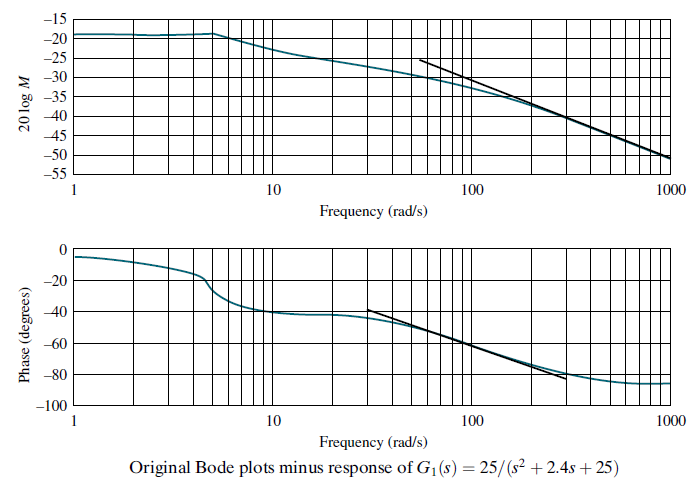
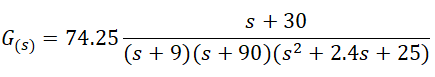
null

Example:


I suggest to visit: Effect of adding a zero to a control system

Source:

  1. Katsuhiko Ogata, Ingeniería de Control Moderno, páginas 65-66.

Written by: Larry Francis Obando – Technical Specialist – Educational Content Writer.

Mentoring Académico / Empresarial / Emprendedores

Copywriting, Content Marketing, Tesis, Monografías, Paper Académicos, White Papers (Español – Inglés)

Escuela de Ingeniería Electrónica de la Universidad Simón Bolívar, Valle de Sartenejas.

Escuela de Ingeniería Eléctrica de la Universidad Central de Venezuela, Caracas.

Escuela de Turismo de la Universidad Simón Bolívar, Núcleo Litoral.

Contact: Caracas, Quito, Guayaquil, Cuenca, España – Telf. +34633129287

Se hacen ejercicios…Atención Inmediata!!

WhatsApp: +34633129287

Twitter: @dademuch

FACEBOOK: DademuchConnection

email: dademuchconnection@gmail.com


Block Diagram, Control System Analysis, Transfer function

Mass-spring-damper rotational system. Problems solved. Catalog 3

The transfer function of a rotational Mass-Spring-Damper System. 

In this PDF guide, the Transfer Function of the exercises that are most commonly used in the mass-spring-damper system classes that are in turn part of control systems, signals and systems, analysis of electrical networks with DC motor, is determined. electronic systems in mechatronics, etc. It is a good resource to also learn how to obtain the block diagram of the system, or the representation in state variables. Request via email – WhatsApp. Payment is provided by PayPal, Credit or debit card. Cost: € 15

Below, the statements of problems solved in this guide.

1. Given the System of Figure 22, find the transfer function Θ(s)/T(s).

null

2. Given the System of Figure 23, find the transfer function Θ(s)/T(s).

null

3. Given the System of Figure 24, find the transfer functions Θ1(s)/T(s)  and Θ2(s)/T(s).

null

4. Find the state-space representation of the system of the previous exercise, Figure 24, taking Θ1(t)  as the output and T(t) as the input. Build the block diagram of the system and determine the transfer function Θ1(s)/T(s).

5. Given the System of Figure 26, find the transfer function ΘL(s)/Tm(s).

null

6. Given the System of Figure 27, find the transfer functions Θ1(s)/Tm(s) and Θ2(s)/Tm(s).

null

7. Given the System of Figure 28, find the transfer functions Θ1(s)/T(s) and Θ2(s)/T(s).

null

8. Given the System of Figure 29, find the transfer function Θ2(s)/T(s).

null

9. Given the System of Figure 30, find the transfer functions  Θ1(s)/T(s) and Θ2(s)/T(s) . Consider: k1=9, k2=3 N-m/rad, b1=8, b2=1 N-m-s/rad, J1=5, J2=3 Kg-m2.

null

10. Find the state-space representation of the system of the previous exercise, Figure 30, taking Θ2(t) as the output and T(t) as the input. Direct Transform the state-space representation obtained into the transfer function Θ2(s)/T(s). Consider k1=9, k2=3 N-m/rad, b1=8, b2=1 N-m-s/rad, J1=5, J2=3 Kg-m2.

11. Find the state-space representation of the system in Figure 32, taking Θ2(t)  as the output and T(t) as the input. Directly, using Matlab, Transform the state-space representation obtained into the transfer function  Θ2(s)/T(s). Consider k1= k2=1 N-m/rad, b1= b2=1 N-m/rad, J=1 Kg-m2.

null

12. Given the System of Figure 33, find the transfer functions  Θ1(s)/Tm(s) and Θ2(s)/Tm(s).

null

Contact:

  • WhatsApp: +34 633129287
  • dademuchconnection@gmail.com

Immediate attention!!..

You may be also interested in:

Made by Prof. Larry Francis Obando – Technical Specialist – Educational Content Writer – Twitter: @dademuch

Mentoring Académico / Emprendedores / Empresarial

Copywriting, Content Marketing, Tesis, Monografías, Paper Académicos, White Papers (Español – Inglés)

Escuela de Ingeniería Eléctrica de la Universidad Central de Venezuela, UCV CCs

Escuela de Ingeniería Electrónica de la Universidad Simón Bolívar, USB Valle de Sartenejas.

Escuela de Turismo de la Universidad Simón Bolívar, Núcleo Litoral.

Contacto: Jaén – España: Tlf. 633129287

Caracas, Quito, Guayaquil, Lima, México, Bogotá, Cochabamba, Santiago.

WhatsApp: +34 633129287

Twitter: @dademuch

FACEBOOK: DademuchConnection

email: dademuchconnection@gmail.com

Control System Analysis, Transfer function

Mass-spring-damper Problems solved. Catalog 2

The transfer function of a Mass-Spring-Damper System. 

In this PDF guide, the Transfer Function of the exercises that are most commonly used in the mass-spring-damper system classes that are in turn part of control systems, signals and systems, analysis of electrical networks with DC motor, is determined. electronic systems in mechatronics, etc. It is a good resource to also learn how to obtain the block diagram of the system, or the representation in state variables. Request via email – WhatsApp. Payment is provided by PayPal, Credit or debit card. Cost: € 15

Below, the statements of problems solved in this guide.

1. Given the System of Figure 12, find the transfer functions Y1(s)/U(s) and Y2(s)/U(s).

null

2. Given the System of Figure 13, find the transfer functions Y1(s)/U(s) and Y2(s)/U(s).

null

3. Given the System of Figure 14, find the transfer functions X1(s)/U(s)  and  X2(s)/U(s).

null

4. Given the System of Figure 15, find the transfer function X2(s)/U(s). Consider k1=1, k2= 15 N/m, b1=4, b2= 16 N-s/m, m1= 8, m2=3  Kg.

null

5. Given the System of Figure 16, find the transfer function X3(s)/U(s). Consider k1=5, k2= 4, k3= 4  N/m, b1=2, b2= 2, b3= 3  N-s/m, m1= 4, m2=5, m3=5  Kg.

null

6.Given the System of Figure 17, find the transfer function X1(s)/U(s). Consider k1=k2= 1 N/m, b1= b2= b3= 1  N-s/m, m1= 2, m2=1, m3=1  Kg. The same exercise is solved with state variables in the next number..

null

7. Find the state-space representation of the system of the previous exercise, Figure 17, taking x1(t) as the output and u(t) as the input. Transform the state-space representation obtained in the transfer function X1(s)/U(s). Consider k1=k2= 1 N/m, b1= b2= b3= 1  N-s/m, m1= 2, m2=1, m3=1  Kg.

8. Given the System of Figure 19, find the transfer function Yh(s)/fup(s). Consider kh=7, ks=8, kave=5  N/m, bf=3, bh= 10  N-s/m, mh=1, mf=2 Kg.

null

9. Given the System of Figure 20, find the transfer functions X2(s)/U(s) and X3(s)/U(s). Consider k1=1, k2=2, k3=3, k4=4 N/m, b1=2,b2= 1,b3= 3 N-s/m, m1=2,m2=1,m3=3  Kg.

null

10. Find the state-space representation of the system in Figure 21, taking x3(t) as the output and u(t) as the input. Transform the state-space representation obtained in the transfer function X3(s)/U(s). Consider k=2 N/m, b1=b2=b3=b4=b5=1 N-s/m, m1=2,m2=1,m3=1  Kg.

null

11. Determine the transfer function X1(s)/ F(s) and the block diagram of the system in Figure 22:

null

Contact:

  • WhatsApp: +34 633129287
  • dademuchconnection@gmail.com

Immediate Attention!!..


You can be interested in:

Elaborado por Prof. Larry Francis Obando – Technical Specialist – Educational Content Writer – Twitter: @dademuch

Mentoring Académico / Emprendedores / Empresarial

Copywriting, Content Marketing, Tesis, Monografías, Paper Académicos, White Papers (Español – Inglés)

Escuela de Ingeniería Eléctrica de la Universidad Central de Venezuela, UCV CCs

Escuela de Ingeniería Electrónica de la Universidad Simón Bolívar, USB Valle de Sartenejas.

Escuela de Turismo de la Universidad Simón Bolívar, Núcleo Litoral.

Contacto: Jaén – España: Tlf. 633129287

Caracas, Quito, Guayaquil, Lima, México, Bogotá, Cochabamba, Santiago.

WhatsApp: +34 633129287

Twitter: @dademuch

FACEBOOK: DademuchConnection

email: dademuchconnection@gmail.com

Bode Diagram, Control System Analysis, Transfer function

Obtaining Transfer Function from Bode Diagram

Bode plots are a convenient presentation of the frequency response data for
the purpose of estimating the transfer function. These plots allow parts of the
transfer function to be determined and extracted, leading the way to further
refinements to find the remaining parts of the transfer function.

Although experience and intuition are invaluable in the process, the following steps are still offered as a guideline:

1. Look at the Bode magnitude and phase plots and estimate the pole-zero configuration of the system. Look at the initial slope on the magnitude plot to determine system type. Look at phase excursions to get an idea of the difference between the number of poles and the number of zeros.
2. See if portions of the magnitude and phase curves represent obvious first- or second-order pole or zero frequency response plots.
3. See if there is any telltale peaking or depressions in the magnitude response plot that indicate an underdamped second-order pole or zero, respectively.
4. If any pole or zero responses can be identified, overlay appropriate ±20 or ±40 dB/decade lines on the magnitude curve or ±45°/decade lines on the phase curve and estimate the break frequencies.For second-order poles or zeros, estimate the damping ratio and natural frequency from the standard curves.
5. Form a transfer function of unity gain using the poles and zeros found. Obtain the frequency response of this transfer function and subtract this response from the previous frequency response (Franklin, 1991). You now have a frequency response of reduced complexity from which to begin the process again to extract more of the system’s poles and zeros. A computer program such as MATLAB is of invaluable help for this step.

Example

Find the transfer function of the subsystem whose Bode plots are shown in Figure 1:

null

Figure 1

Let us first extract the underdamped poles that we suspect, based on the peaking in the magnitude curve.We estimate the natural frequency to be near the peak frequency, or approximately 5 rad/s. From Figure 1, we see a peak of about 6.5 dB, which translates into a damping ratio of about ζ=0,24. The unity gain second-order function is thus:

null

The frequency response plot of this function is made and subtracted from the previous
Bode plots to yield the response in Figure 2:

null

Figure 2

Overlaying a -20 dB/decade line on the magnitude response and a -45°/decade line on the phase response, we detect a final pole. From the phase response, we estimate the break frequency at 90 rad/s. Subtracting the response of G2(s)=90/(s+90) from the previous response yields the response in Figure 3.

null

Figure 3

Figure 3 has a magnitude and phase curve similar to that generated by a lag function. We draw a -20 dB/decade line and fit it to the curves. The break frequencies are read from the figure as 9 and 30 rad/s. A unity gain transfer function containing a pole at -9 and a zero at -30 is G3(s)=0.3(s+30)/(s+9). Upon subtraction of G1(s)G2(s)G3(s), we find the magnitude frequency response flat ±1 dB and the phase response flat at -3± 5°. We thus conclude that we are finished extracting dynamic transfer functions as:

null

It is interesting to note that the original curve was obtained from the function:

null

Sources:

  1. Modern_Control_Engineering, Ogata 4t
  2. Control Systems Engineering, Nise
  3. Sistemas de Control Automatico, Kuo

Literature review by:

Prof. Larry Francis Obando – Technical Specialist – Educational Content Writer

Resolving problems!!

WhatsApp:  +34633129287  Immediate attention!!

Twitter: @dademuch

Copywriting, Content Marketing, Tesis, Monografías, Paper Académicos, White Papers (Español – Inglés)

Escuela de Ingeniería Electrónica de la Universidad Simón Bolívar, USB Valle de Sartenejas.

Escuela de Ingeniería Eléctrica de la Universidad Central de Venezuela, UCV CCs

Escuela de Turismo de la Universidad Simón Bolívar, Núcleo Litoral.

Contacto: España. +34633129287

Caracas, Quito, Guayaquil, Cuenca. 

WhatsApp:  +34633129287   +593998524011  

Twitter: @dademuch

FACEBOOK: DademuchConnection

email: dademuchconnection@gmail.com