Criterio de Nyquist, Digital Signal Processing, Procesamiento de señales digitales, Señales y Sistemas, Sistemas LDCID

Aliasing – sampling with a periodic impulse train

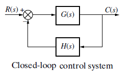
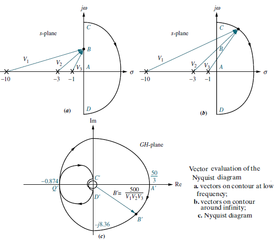
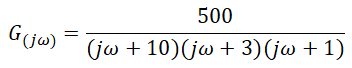
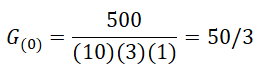
Sampling – Chapter One

Sampling with a periodic impulse train.

The Periodic Sampling is the typical method of obtaining a Discrete-time representation of a Continuous-time signal, wherein a sequence of samples x[n] is obtained from a Continuous-time signal xc(t), according to the relation:

Where T is the sampling period and its reciprocal, Fs=1/T, is the sampling frequency. We refer to a system that implements the operation of equation (1) as an ideal continuous-to-discrete-time (C/D) converter.

To derive the frequency-domain relation between the input and output of an ideal C/D converter, first consider the conversion of xc(t) to xs(t) through modulation of the periodic impulse train:

We modulate the periodic impulse s(t) train with xc(t), obtaining:

Through the “sifting property” of the impulse function, xs(t) can be expressed as:

Figure 4.2(a) is strictly a mathematical representation that is convenient for gaining insight into sampling in both time domain and frequency domain. It is not a close representation of any physical circuit or system. This representation leads to a simple derivation of a key result and to a number of important insights that are difficult to obtain from a forma derivation based on manipulation of Fourier Transform formulas.

The sampling operation is generally not invertible; i.e., given the output x[n], it is not possible to reconstruct xc(t), the input to the sampler, since many continuous-time signals can produce the same output sequence. The inherent ambiguity in sampling is a fundamental issue in signal processing. Fortunately, it is possible to remove the ambiguity by restricting the input signals that go into the sampler.

Figure 4.2 (b) shows a continuous-time signal xc(t) and the results of impulse train sampling for two different sampling rates. Figure 4.2 (c) depicts the corresponding output sequences. The essential difference between xs(t) and x[n] is that xs(t) is, in a sense, a continuous-time signal that is zero except at integer multiples of T. The sequence x[n], on the other hand, is indexed on the integer variable n, which in effect introduces a time normalization; i.e., the sequence of numbers x[n] contains no explicit information about the sampling rate. Furthermore, the samples of xc(t) are represented by finite numbers in x[n] rather than as an area of impulses, as with xs(t).

Sampling principle.

A band-limited signal xc(t) with bandwidth Fo can be reconstructed from its sample values x[n]=xc(nT), if the sample frequency Fs=1/Ts is greater than twice the bandwidth Fo of xc(t):

Otherwise, aliasing would result in x[n]. The sampling rate of 2Fo  for an analog band-limited signal is called the Nyquist rate.

Note: according to Nyquist criteria, after xc(t) is sampled, the highest analog frequency that x[n] represents must be Fs/2 (i.e. ω=π).

Band-limited signal.

A continuous-time signal xa(t) is band-limited if there exist a finite radian frequency Ωo such that the CT-Fourier Transform Xa(jΩ) is zero for |Ω|> Ωo:

The frequency Fo is called the signal bandwidth in Hz.

Aliasing.

Let xa(t) be an analog (absolutely integrable) signal. The continuous-time Fourier Transform (CTFT) of xa(t) is:

Meanwhile:

In consequence, it can be shown that the discrete-time Fourier Transform (DTFT) of x[n] is a countable sum of amplitude-scaled, frequency-scaled, and translated version of the Fourier Transform Xa(jΩ):

This relation is known as the aliasing formula. The analog and digital frequencies are related through Ts:

While the sampling frequency Fs is given by:

When we want to express the sampling frequency in radians per second, we also use:

The graphical illustration of the aliasing phenomena is given by Figure 3.10:

Combining this we obtain this simple aliasing principle:

Example 3.17

The analog signal xa(t) is sampled at Fs to obtain the discrete-time signal x[n]. Determine x[n] and its corresponding DTFT.

Solution:

First, we must identify the highest frequency in xa(t). That will be F0:

Since  Fs <2 F0, there will be aliasing in x[n] after sampling. i.e., we will get the following case:

The sampling interval is:

Hence, we have:

That is:

Note that the highest digital frequency of x[n] is 1.75π, which is outside the Nyquist interval –π<ω<π, signifying that aliasing will occur. From the periodicity property of digital sinusoidal sequences, we know that x[n] will be repeated every 2π. So, the alias of  x[n] can be determined by:

Using Euler’s identity:

From table 3.1 and the DTFT properties, the DTFT of x[n] is:

The plot of X(e) is shown in Figure 3.15.

Figure 3.15. The Fourier Transform of x[n].

Source:

Ingel V.; Proakis J. Digital Signal processing using Matlab (p 81)

Oppenheim A.; Schafer R.; Buck J. Discrete Time Signal Processing (p 141)

Book Review by Larry Obando – Electrical Engineering –

Universidad Simón Bolívar – Universidad Central de Venezuela

Mathematical Modeling and Simulation Services – whatsapp +34633129287

Análisis de sistemas de control, Criterio de Nyquist

Estabilidad vía Nyquist Diagrama – El criterio de Nyquist

El criterio de Nyquist puede decirnos si el sistema es estable o inestable al determinar cuántos polos del sistema a lazo cerrado de la Figura 1, se encuentran en el semiplano derecho:

null

Figura 1

Considere el contorno A definido en el plano s de la figura 2:

null

Figura 2

Si un contorno, A, que rodea todo el semiplano derecho del lugar de raíces del sistema determinado por la ecuación característica 1+ G(s)H(s), se mapea a través de G(s)H(s), entonces el número de polos del sistema a lazo cerrado, Z, en el semiplano derecho es igual al número de polos del sistema a lazo abierto, P, que están en el semiplano derecho menos el número de revoluciones en sentido antihorario, N, alrededor de -1+j0 del mapa; es decir, Z:

null

En consecuencia, para lograr estabilidad, Z debe ser igual a cero.

Ejemplo:

null

Step 1. Find the open-loop transfer function G(s)H(s) of the system.

Consider the closed-loop control system as follows:

null

The system characteristic equation is as follows:

null

The factor form of this characteristic equation is:

null

To determine the previous factor form:

null

Where the open-loop transfer function G(s)H(s) of the system is:

null

Step 2. Use Command Window of Matlab to draw the Nyquist Diagram, applying the following commands:

>> s=tf(‘s’);

>> G=10/(s^3+2*s^2+5*s);

>> nyquist(G);

null

null

We can see at the previous Diagram that for:

null

To reach stability, Z must be equal to zero:

null

Recalling that the poles of 1+ G(s)H(s), are the same as the poles of G(s)H(s), the open-loop system, we can determine P, the number of open-loop poles enclosed by the contour A from:

null

null

A detour around the poles on the contour is required:

null

In the Nyquist Diagram obtained for the system of Task 2, the point -1+j0 is highlighted in red:

null

We can see that N=0, so:

null

However, the Nyquist diagram intersects the real axis at -1+j0. Hence, according to the Nyquist Criteria, the system is marginally stable.

Fuentes:

  1. Modern_Control_Engineering, Ogata 4t
  2. Control Systems Engineering, Nise
  3. Sistemas de Control Automatico, Kuo

Revisión literaria hecha por:

Prof. Larry Francis Obando – Technical Specialist – Educational Content Writer

Se hacen trabajos, se resuelven ejercicios!!

WhatsApp:  +34633129287  Atención Inmediata!!

Twitter: @dademuch

Copywriting, Content Marketing, Tesis, Monografías, Paper Académicos, White Papers (Español – Inglés)

Escuela de Ingeniería Electrónica de la Universidad Simón Bolívar, USB Valle de Sartenejas.

Escuela de Ingeniería Eléctrica de la Universidad Central de Venezuela, UCV CCs

Escuela de Turismo de la Universidad Simón Bolívar, Núcleo Litoral.

Contacto: España. +34633129287

Caracas, Quito, Guayaquil, Cuenca. 

WhatsApp:  +34633129287   +593998524011  

Twitter: @dademuch

FACEBOOK: DademuchConnection

email: dademuchconnection@gmail.com

Análisis de sistemas de control, Criterio de Nyquist

El diagrama de Nyquist

El diagrama de Nyquist, también es conocido como «La Traza Polar» de una función de transferencia senoidal G(jω), es una gráfica de la magnitud de G(jω) contra el ángulo de fase de G(jω) en coordenadas polares, conforme ω varía de cero a infinito. Por tanto, El diagrama de Nyquist es el lugar geométrico de los vectores:

null
conforme ω varía de cero a infinito. Observe que, en las gráficas polares, los ángulos de fase son positivos (negativos) si se miden en el sentido contrario de las manecillas del reloj (en el sentido de las manecillas) a partir del eje real positivo.

La siguiente figura muestra un ejemplo de un diagrama de Nyquist:

null

Todos los puntos de la traza polar de G(jω) representan el punto terminal de un vector en un valor determinado de ω. Las proyecciones de G(jω) en los ejes real e imaginario son sus componentes real e imaginaria. La magnitud y el ángulo de fase de G(jω) deben calcularse directamente para cada frecuencia ω con el propósito de construir trazas polares.

Conceptualmente, el diagrama de Nyquist se traza sustituyendo los puntos del «contorno» que encierra el semiplano derecho, en la función G(s)H(s). Este proceso se llama mapeo (mapping):

null

Consideremos el sistema de control a lazo cerrado de la Figura 1:

null

Figura 1

Entonces, en el Diagrama de Nyquist, el contorno que encierra el semiplano derecho, que se muestra en la Figura 2, puede mapearse a través de la función G(s)H(s), derivada de la Figura 1, sustituyendo puntos a lo largo del contorno en la función G(s)H(s).

null

Figura 2

Estabilidad vía el Diagrama de Nyquist

Si un contorno, A, que rodea todo el semiplano derecho del lugar de raíces del sistema determinado por la ecuación característica 1+ G(s)H(s), se mapea a través de G(s)H(s), entonces el número de polos del sistema a lazo cerrado, Z, en el semiplano derecho, es igual al número de polos del sistema a lazo abierto, P, que están en el semiplano derecho menos el número de revoluciones en sentido antihorario, N, alrededor de -1+j0 del plano complejo ; es decir, Z:

null

Por tanto, para lograr un sistema estable a lazo cerrado, Z debe ser igual a cero.

Este «mapping» es llamado El Diagrama de Nyquist , o Nyquist plot, de G(s)H(s). Para más información y ejemplos ver: Criterio de Nyquist para estabilidad

Ejemplo 

Considere el sistema de control cuyo esquema y diagrama de bloques se muestran en la siguiente Figura 3:

null

Figura 3

Conceptualmente, el diagrama de Nyquist se representa sustituyendo los puntos del contorno que se muestran en la Figura 4(a) en G(s)H(s):

null

Cada Polo y cada Zero de G(s)H(s) que se muestra en la Figura 3(b) es un vector en la Figura 4(a) y 4(b). El vector resultante, , encontrado en cualquier punto a lo largo del contorno, es en general el producto de los vectores Zero dividido por el producto de los vectores Polo (ver Figura 4 (c)). Por lo tanto, la magnitud de la resultante es el producto de las longitudes Zero dividido por el producto de las longitudes de los Polos, y el ángulo de la resultante es la suma de los ángulos Zero menos la suma de los ángulos de los Polos.

null

Figura 4

El mapeo del punto A al punto C también puede explicarse analíticamente. Desde
A a C, la colección de puntos a lo largo del contorno es imaginaria. Por lo tanto, de A a C,
G(s)H(s)=G(s)*1=G(s)=G(jω), o de la Figura 3(b):

null

A frecuencia igual cero:

null

Por lo tanto, el diagrama de Nyquist comienza en 50/3 en un ángulo de . A medida que ω aumenta, la parte real sigue siendo positiva, y la parte imaginaria sigue siendo negativa.

En null la parte real se vuelve negativa. En null, el diagrama de Nyquist cruza el eje real negativo ya que el término imaginario va a cero. El valor real en el cruce del eje, punto Q en la Figura 4 (c), es -0.874. Continuando hacia, la parte real es negativa, y la parte imaginaria es positiva. A frecuencia infinita:

null

o cero a los 90°. aproximadamente.

Alrededor del semicírculo infinito desde el punto C hasta el punto D que se muestra en la Figura 4(b), los vectores giran en sentido horario, cada uno 180°. Por lo tanto, la resultante sufre una rotación en sentido antihorario de 3×180, comenzando en el punto C’ y terminando en el punto D’ de la Figura 4 (c).

Diagrama de Nyquist con Matlab

Considere la siguiente función de transferencia a lazo abierto:

null

Para elaborar el Diagrama de Nyquist, podemos utilizar los siguientes comandos en el command window de Matlab:

>> s=tf(‘s’)

>> G=1/(s^2+0.8*s+1)

>> nyquist(G)

Esta línea de comandos genera la siguiente gráfica:

null

Podemos obtener información sobre puntos de interés en el diagrama de Nyquist haciendo clik una vez sobre el punto de interés en el contorno:

null

Siguiente:

Fuentes:

  1. Modern_Control_Engineering, Ogata 4t
  2. Control Systems Engineering, Nise
  3. Sistemas de Control Automatico, Kuo

Revisión literaria hecha por:

Prof. Larry Francis Obando – Technical Specialist – Educational Content Writer

Se hacen trabajos, se resuelven ejercicios!!

WhatsApp:  +34633129287  Atención Inmediata!!

Twitter: @dademuch

Copywriting, Content Marketing, Tesis, Monografías, Paper Académicos, White Papers (Español – Inglés)

Escuela de Ingeniería Electrónica de la Universidad Simón Bolívar, USB Valle de Sartenejas.

Escuela de Ingeniería Eléctrica de la Universidad Central de Venezuela, UCV CCs

Escuela de Turismo de la Universidad Simón Bolívar, Núcleo Litoral.

Contacto: España. +34633129287

Caracas, Quito, Guayaquil, Cuenca. 

WhatsApp:  +34633129287   +593998524011  

Twitter: @dademuch

FACEBOOK: DademuchConnection

email: dademuchconnection@gmail.com