Fiabilidad y validez de instrumentos de medición en investigación cuantitativa

Recolectar los datos implica elaborar un plan detallado de procedimientos que conduzcan a reunir datos con un propósito específico. Este plan incluye determinar:

1. ¿Cuáles son las fuentes de donde se obtendrán los datos?
2. ¿Dónde se localizan tales fuentes?
3. ¿De qué forma vamos a preparar los datos para analizarlos?
4. ¿De qué recursos disponemos?

La siguiente es una guía para diseñar dichos instrumentos: Fiabilidad de los instrumentos.

Revisión literaria hecha por:

Prof. Larry Francis Obando – Technical Specialist – Educational Content Writer

Se hacen trabajos!!

WhatsApp:  +34633129287  Atención Inmediata!!

Twitter: @dademuch

Copywriting, Content Marketing, Tesis, Monografías, Paper Académicos, White Papers (Español – Inglés)

Escuela de Ingeniería Eléctrica de la Universidad Central de Venezuela, UCV CCs

Escuela de Ingeniería Electrónica de la Universidad Simón Bolívar, USB Valle de Sartenejas.

Escuela de Turismo de la Universidad Simón Bolívar, Núcleo Litoral.

Contacto: España. +34633129287

Caracas, Quito, Guayaquil, Cuenca. 

WhatsApp:  +34633129287   +593998524011  

Twitter: @dademuch

FACEBOOK: DademuchConnection

email: dademuchconnection@gmail.com

Obtaining Transfer Function from Bode Diagram

Bode plots are a convenient presentation of the frequency response data for
the purpose of estimating the transfer function. These plots allow parts of the
transfer function to be determined and extracted, leading the way to further
refinements to find the remaining parts of the transfer function.

Although experience and intuition are invaluable in the process, the following steps are still offered as a guideline:

1. Look at the Bode magnitude and phase plots and estimate the pole-zero configuration of the system. Look at the initial slope on the magnitude plot to determine system type. Look at phase excursions to get an idea of the difference between the number of poles and the number of zeros.
2. See if portions of the magnitude and phase curves represent obvious first- or second-order pole or zero frequency response plots.
3. See if there is any telltale peaking or depressions in the magnitude response plot that indicate an underdamped second-order pole or zero, respectively.
4. If any pole or zero responses can be identified, overlay appropriate ±20 or ±40 dB/decade lines on the magnitude curve or ±45°/decade lines on the phase curve and estimate the break frequencies.For second-order poles or zeros, estimate the damping ratio and natural frequency from the standard curves.
5. Form a transfer function of unity gain using the poles and zeros found. Obtain the frequency response of this transfer function and subtract this response from the previous frequency response (Franklin, 1991). You now have a frequency response of reduced complexity from which to begin the process again to extract more of the system’s poles and zeros. A computer program such as MATLAB is of invaluable help for this step.

Example

Find the transfer function of the subsystem whose Bode plots are shown in Figure 1:

Figure 1

Let us first extract the underdamped poles that we suspect, based on the peaking in the magnitude curve.We estimate the natural frequency to be near the peak frequency, or approximately 5 rad/s. From Figure 1, we see a peak of about 6.5 dB, which translates into a damping ratio of about ζ=0,24. The unity gain second-order function is thus:

The frequency response plot of this function is made and subtracted from the previous
Bode plots to yield the response in Figure 2:

Figure 2

Overlaying a -20 dB/decade line on the magnitude response and a -45°/decade line on the phase response, we detect a final pole. From the phase response, we estimate the break frequency at 90 rad/s. Subtracting the response of G2(s)=90/(s+90) from the previous response yields the response in Figure 3.

Figure 3

Figure 3 has a magnitude and phase curve similar to that generated by a lag function. We draw a -20 dB/decade line and fit it to the curves. The break frequencies are read from the figure as 9 and 30 rad/s. A unity gain transfer function containing a pole at -9 and a zero at -30 is G3(s)=0.3(s+30)/(s+9). Upon subtraction of G1(s)G2(s)G3(s), we find the magnitude frequency response flat ±1 dB and the phase response flat at -3± 5°. We thus conclude that we are finished extracting dynamic transfer functions as:

It is interesting to note that the original curve was obtained from the function:

Sources:

1. Modern_Control_Engineering, Ogata 4t
2. Control Systems Engineering, Nise
3. Sistemas de Control Automatico, Kuo

Literature review by:

Prof. Larry Francis Obando – Technical Specialist – Educational Content Writer

Resolving problems!!

WhatsApp:  +34633129287  Immediate attention!!

Twitter: @dademuch

Copywriting, Content Marketing, Tesis, Monografías, Paper Académicos, White Papers (Español – Inglés)

Escuela de Ingeniería Electrónica de la Universidad Simón Bolívar, USB Valle de Sartenejas.

Escuela de Ingeniería Eléctrica de la Universidad Central de Venezuela, UCV CCs

Escuela de Turismo de la Universidad Simón Bolívar, Núcleo Litoral.

Contacto: España. +34633129287

Caracas, Quito, Guayaquil, Cuenca. 

WhatsApp:  +34633129287   +593998524011  

Twitter: @dademuch

FACEBOOK: DademuchConnection

email: dademuchconnection@gmail.com

 

Función de transferencia a partir del diagrama de Bode.

Los gráficos de Bode son una presentación conveniente de los datos de respuesta de frecuencia para el propósito de estimar la función de transferencia. El Diagrama de Bode permite determinar y extraer partes de la función de transferencia, lo que abrirá el camino a más cálculos para encontrar las partes restantes de dicha función.

Aunque la experiencia y la intuición son invaluables en el proceso, los siguientes pasos  ofrecen una guía:

1. Observe las gráficas de magnitud y fase de Bode y estime la configuración de polos y zeros del sistema. Observar la pendiente inicial en el diagrama de magnitud para determinar el tipo de sistema. Observar las excursiones de fase para tener una idea de la diferencia entre el número de polos y el número de zeros.
2. Vea si partes de las curvas de magnitud y fase representan gráficas obvias de respuesta de frecuencia de polo o zero de primer o segundo orden.
3. Observar si hay algún pico revelador o depresiones en la gráfica de magnitud que indique un polo de segundo orden o zero amortiguado, respectivamente.
4. Si alguna respuesta típica de un polo o un zero puede ser identificada, superponer líneas apropiadas de ± 20 o ± 40 dB / década en la curva de magnitud o líneas de ±45°/década en la curva de fase y estimar las frecuencias de ruptura. Para polos o zeros de segundo orden, calcule la relación de amortiguamiento y la frecuencia natural a partir de las curvas estándar.

5. Diseñar una función de transferencia de ganancia unitaria utilizando los polos y zeros encontrados. Obtenga la respuesta de frecuencia de esta función de transferencia y reste esta respuesta de la respuesta de frecuencia anterior, con la que comenzó el ejercicio. Ahora tiene una respuesta de frecuencia de complejidad reducida a partir de la cual comenzar el proceso nuevamente para extraer más información sobre los polos y ceros del sistema. Un programa de computadora como MATLAB es de gran ayuda para este paso.

Example

Encontrar la función de transferencia del sistema cuyo diagrama de Bode se muestra en la Figura 1:

Figura 1

Primero extraigamos los polos subamortigados, basados en el pico en la curva de magnitud. Estimamos que la frecuencia natural está cerca de la frecuencia pico, o aproximadamente 5 rad/s. De la Figura 1, podemos ver un pico alrededor de 6.5 dB, que se interpreta como un factor de amortiguamiento ζ=0,24. La función de transferencia estándar de un sistema de segundo orden con ganancia unitaria es:

Se restan los diagramas de Bode en la Figura 2:

Figura 2

Al superponer una línea de -20 dB/decade en la respuesta de magnitud y una línea de -45°/decade en la respuesta de fase, detectamos un polo final. A partir de la respuesta de fase, estimamos la frecuencia de ruptura a 90 rad/s. Restando la respuesta de G2(s)=90/(s+90) de la respuesta anterior se obtiene la respuesta en la Figura 3.

Figura 3

La figura 3 tiene una curva de magnitud y fase similar a la generada por una función de retraso. Dibujamos una línea de -20 dB/decade y la ajustamos a las curvas. Las frecuencias de ruptura se leen de la figura como 9 y 30 rad/s. Una función de transferencia de ganancia unitaria que contiene un polo en -9 y un cero en -30 es G3(s)=0.3(s+30)/(s+9). Al restar G1(s)G2(s)G3(s), encontramos la respuesta de frecuencia de magnitud plana ± 1 dB y la respuesta de fase plana a -3 ± 5 °. Por lo tanto, concluimos que hemos terminado de extraer las funciones de transferencia dinámica, la cual es:

Es interesante notar que la curva original se obtuvo de la función:

Fuentes:

1. Modern_Control_Engineering, Ogata 4t
2. Control Systems Engineering, Nise
3. Sistemas de Control Automatico, Kuo

Revisión literaria hecha por:

Prof. Larry Francis Obando – Technical Specialist – Educational Content Writer

Se hacen trabajos, se resuelven ejercicios!!

WhatsApp:  +34633129287  Atención Inmediata!!

Twitter: @dademuch

Copywriting, Content Marketing, Tesis, Monografías, Paper Académicos, White Papers (Español – Inglés)

Escuela de Ingeniería Electrónica de la Universidad Simón Bolívar, USB Valle de Sartenejas.

Escuela de Ingeniería Eléctrica de la Universidad Central de Venezuela, UCV CCs

Escuela de Turismo de la Universidad Simón Bolívar, Núcleo Litoral.

Contacto: España. +34633129287

Caracas, Quito, Guayaquil, Cuenca. 

WhatsApp:  +34633129287   +593998524011  

Twitter: @dademuch

FACEBOOK: DademuchConnection

email: dademuchconnection@gmail.com

El diagrama de Bode – Gráfica de respuesta en frecuencia de un sistema de control.

El diagrama de Bode es el trazado de la respuesta de frecuencia de un sistema con gráficos de magnitud y fase separados. Las curvas de respuesta en frecuencia, de magnitud y  de fase como funciones de log ω se denominan Diagramas de Bode. El dibujar diagramas de Bode se puede simplificar porque se pueden aproximar como una secuencia de líneas rectas. Las aproximaciones en línea recta simplifican la evaluación de la de magnitud y  de fase de la respuesta en frecuencia.

Cuando elaboramos las gráficas de magnitud y  de fase por separado, la gráfica de la curva de magnitud puede tener el eje de las ordenadas en decibeles (dB) vs. log ω en el eje de las abscisas, donde dB = 20 log M.

Ejemplo

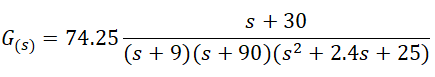
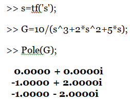
Graficar el Diagrama de Bode para la respuesta en frecuencia del sistema descrito por la función de Transferencia G(s):

Factores Básicos de G(jω)H(jω)

La ventaja principal de usar una traza logarítmica es la facilidad relativa de graficar las curvas de la respuesta en frecuencia. Los factores básicos que suelen ocurrir en una función de transferencia arbitraria G(jω)H(jω) son:

1. La ganancia K
2. Los factores de integral y de derivada ,
3. Los factores de primer orden ,
4. Los factores cuadráticos .

Una vez que nos familiarizamos con las trazas logarítmicas de estos factores básicos, es posible utilizarlas con el fin de construir una traza logarítmica compuesta para cualquier forma de G(jω)H(jω), trazando las curvas para cada factor y agregando curvas individuales en forma gráfica, ya que agregar los logaritmos de las ganancias corresponde a multiplicarlos entre sí.

El proceso de obtener la traza logarítmica se simplifica todavía más mediante aproximaciones asintóticas para las curvas de cada factor.

GANANCIA

La ganancia K. Un número mayor que la unidad tiene un valor positivo en decibeles, en tanto que un número menor que la unidad tiene un valor negativo.

La curva de magnitud logarítmica para una ganancia constante K es una recta horizontal cuya magnitud es de 20 log K decibeles. El ángulo de fase de la ganancia K es cero.

El efecto de variar la ganancia K en la función de transferencia es que sube o baja la curva de magnitud logarítmica de la función de transferencia en la cantidad constante correspondiente, pero no afecta la curva de fase.

POLOS Y CEROS EN EL ORIGEN

Factores de integral y de derivada(polos y ceros en el origen).

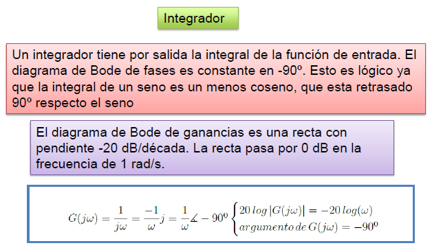
Supongamos el factor 1/s en una función de transferencia cualquiera. El factor 1/s es un integrador. Es decir, la salida de ese sistema es la integral de la entrada. Al sustituir s=jω obtenemos el factor l/jω. La magnitud logarítmica de l/jω en decibeles es:

El ángulo de fase de l/jω es constante e igual a -90^°.

En las trazas de Bode, las razones de frecuencia se expresan en términos de octavas o décadas. Una octava es una banda de frecuencia de ω₁ a 2ω₁, en donde ω₁ es cualquier frecuencia. Una década es una banda de frecuencia de ω₁ a 10ω₁, en donde, otra vez, ω₁ es cualquier frecuencia. (En la escala logarítmica del papel semi logarítmico, cualquier razón de frecuencia determinada se representa mediante la misma distancia horizontal. Por ejemplo, la distancia horizontal de ω=1  a ω=10  es igual a la de ω=3  a ω=30.

Si se gráfica la magnitud logarítmica de -20logω dB contra ω en una escala logarítmica,  se obtiene una recta. Para trazar esta recta, necesitamos ubicar un punto (0 dB, ω= 1) en ella. Dado que:

La pendiente m de la recta para l/jω es de:

El ángulo de fase del factor l/jω es constante e igual a -90^°

De igual forma, el factor s es un derivador. Es decir, la salida de ese sistema es la derivada de la entrada. La magnitud logarítmica de s=jω en decibeles es::

La pendiente m de la recta para jω es de:

El ángulo de fase del factor jω es constante e igual a 90^°

La siguiente figura muestra curvas de respuesta en frecuencia para l/jω y jω, respectivamente.

Observar que ambas magnitudes logarítmicas se vuelven iguales a 0 dB en ω=1. (Cortan al eje de abcisas en ω=1)

Por tanto, si la función de transferencia contiene el factor (l/jω)ⁿ o (jω)ⁿ , la magnitud logarítmica se convierte, respectivamente, en:

Por tanto, las pendientes de las curvas de magnitud logarítmica para los factores  (l/jω)ⁿ y (jω)ⁿ son -20n dB/década y 20n dB/década, respectivamente.

El ángulo de fase de (l/jω)ⁿ es igual a -90^°n durante todo el rango de frecuencia, en tanto que el ángulo de fase de (jω)ⁿ es igual a 90^°n en todo el rango de frecuencia. Las curvas de magnitud pasarán por el punto (0 dB,  ω= 1).

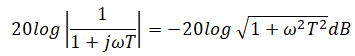
Factores de primer orden. La magnitud logarítmica del factor de primer orden l/(1+jωT) en decibeles es:

Para frecuencias bajas, tales que ω<<1/T, la magnitud logarítmica se aproxima mediante:

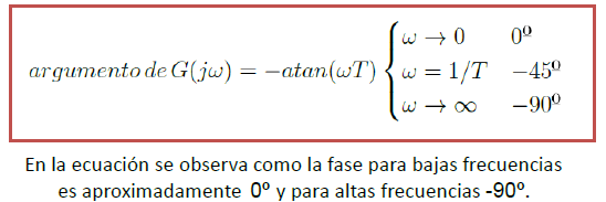
Por tanto, la curva de magnitud logarítmica para frecuencias bajas en este factor es la línea 0 dB constante. Para frecuencias altas, tales que :

Ésta última es una expresión aproximada para el rango de altas frecuencias. En ω=1/T , la magnitud logarítmica es igual a 0 dB; en ω=10/T, la magnitud logarítmica es de -20 dB. Por tanto, el valor de -20logωT dB  disminuye en 20 dB para todas las décadas de ω. De esta forma, para ω>>1/T, la curva de magnitud logarítmica es una línea recta con una pendiente de -20 dB/década (o -6 dB/octava).

Nuestro análisis muestra que la representación logarítmica de la curva de respuesta en frecuencia del factor l/(1+jωT) se aproxima mediante dos asíntotas (líneas rectas), una de las cuales es una recta de 0 dB para el rango de frecuencia 0<ω<1/T  y la otra es una recta con una pendiente de -20 dB/década (o -6 dB/octava) para el rango de frecuencia 1/T<ω<∞. La frecuencia en la cual las dos asíntotas se encuentran se denomina frecuencia de esquina o frecuencia de corte. Para el factor l/(1+jωT), la frecuencia ω=1/T es la frecuencia de esquina, dado que en ese punto ambas asíntotas tienen el mismo valor.

La función de transferencia de l/(1+jωT) tiene las características de un filtro pasa-baja. Para frecuencias por encima de ω=1/T, la magnitud logarítmica disminuye rápidamente hacia –infinito. Esto se debe, en esencia, a la presencia de la constante de tiempo. En el filtro pasa-baja, la salida sigue fielmente a la entrada sinusoidal a bajas frecuencias. Pero, conforme aumenta la frecuencia de entrada, la salida no puede seguir a la entrada debido a que se necesita cierta cantidad de tiempo para que el sistema aumente en magnitud. Por tanto, para altas frecuencias, la amplitud de la salida tiende a cero y el ángulo de fase tiende a -90°. En este aso, si la entrada posee muchos armónicos, las componentes de baja frecuencia se reproducen fielmente en la salida, mientras que las componentes de alta frecuencia se atenúan en amplitud y cambian en fase. Por tanto, un elemento de primer orden produce una duplicación exacta, o casi exacta, sólo para fenómenos constantes o que varían lentamente.

Resumen para polo simple:

Una ventaja de las trazas de Bode es que, para factores recíprocos, por ejemplo, el factor 1+jωT, las curvas de magnitud logarítmica y de ángulo de fase sólo necesitan cambiar de signo. Por tanto, la pendiente de la asíntota de alta frecuencia de 1+jωT es 20 dB/década, y el ángulo de fase varía de 0^°  a 90^°  conforme la frecuencia ω se incrementa de cero a infinito., como se puede ver en la siguiente Figura:

Se puede calcular el error en la curva de magnitud provocado por el uso de las asíntotas. El error máximo ocurre en la frecuencia de esquina y es aproximadamente igual a -3 dB debido a que:

El error es simétrico con respecto a la frecuencia de esquina. El error en decibelios implícito al usa la expresión asintótica para la curva de respuesta en frecuencia de l/(1+jωT)  se muestra en figura siguiente:

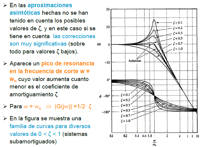
CUADRÁTICOS

Factores cuadráticos. Los sistemas de control suelen tener factores cuadráticos de la forma:

Si ζ>1, este factor cuadrático se expresa como un producto de dos factores de primer orden con polos reales. Si 0<ζ<1, este factor cuadrático es el producto de dos factores complejos conjugados.

La curva asintótica de respuesta en frecuencia para se obtiene del modo siguiente. Dado que:

para frecuencias bajas tales que ω<<ω_n, la magnitud logarítmica se convierte en:

Por tanto, la asíntota de frecuencia baja es una recta horizontal en 0 dB. Para frecuencias altas tales que ω>>ω_n, la magnitud logarítmica se vuelve:

La ecuación para la asíntota de alta frecuencia es una recta con pendiente de -40dB/década, dado que:

La asíntota de alta frecuencia intercepta la de baja frecuencia en ω=ω_n, dado que en esta frecuencia:

Esta frecuencia ω_n es la frecuencia de esquina para el factor cuadrático considerado.

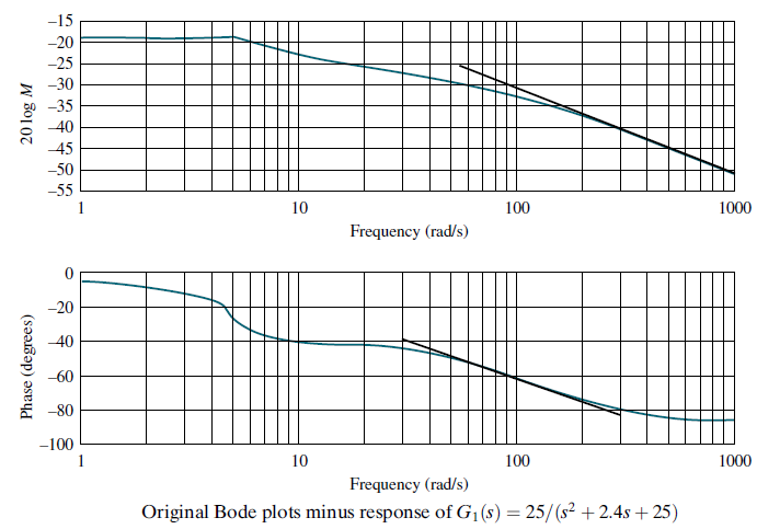
Ejemplo:

ANEXO 1.

ANEXO 2.

ANEXO 3.

ANEXO 4.

Te puede interesar:

• Formulario de examen resuelto – Diagrama de Bode
• Respuesta forzada a una entrada exponencial utilizando el Diagrama de Bode

Fuentes:

1. Modern_Control_Engineering, Ogata 4t
2. Control Systems Engineering, Nise
3. Sistemas de Control Automatico, Kuo

Revisión literaria hecha por:

Prof. Larry Francis Obando – Technical Specialist – Educational Content Writer

Se hacen trabajos, se resuelven ejercicios!!

WhatsApp:  +34633129287  Atención Inmediata!!

Twitter: @dademuch

Copywriting, Content Marketing, Tesis, Monografías, Paper Académicos, White Papers (Español – Inglés)

Escuela de Ingeniería Electrónica de la Universidad Simón Bolívar, USB Valle de Sartenejas.

Escuela de Ingeniería Eléctrica de la Universidad Central de Venezuela, UCV CCs

Escuela de Turismo de la Universidad Simón Bolívar, Núcleo Litoral.

Contacto: España. +34633129287

Caracas, Quito, Guayaquil, Cuenca. 

WhatsApp:  +34633129287  

Twitter: @dademuch

FACEBOOK: DademuchConnection

email: dademuchconnection@gmail.com

The Bode Diagrams – Plotting of the frequency response of a control system.

The Bode Diagrams is the plotting of the frequency response of a system with separate magnitude and phase plots. The log-magnitude and phase frequency response curves as functions of log ω  are called Bode plots or Bode diagrams. Sketching Bode plots can be simplified because they can be approximated as a sequence of straight lines. Straight-line approximations simplify the evaluation of the magnitude and phase frequency response.

When plotting separate magnitude and phase plots, the magnitude curve can be plotted in decibels (dB) vs. log ω, where dB = 20 log M. Meanwhile, the phase curve is plotted as phase angle vs. log ω.

Example

Plot The Bode Diagram for the frequency response of the characterized by the system Transfer Function G(s):

Basic Factors of G(jω)H(jω)

The main advantage of using a logarithmic trace is the relative ease of plotting the frequency response curves. The basic factors that are frequent in an arbitrary transfer function G(jω)H(jω) are:

1. The gain K
2. Integral and derivative factors ,
3. First order factors ,
4. The quadratic factors .

Once we become familiar with the logarithmic traces of these basic factors, it is possible to use them in order to construct a composite logarithmic trace for any form of G(jω)H(jω), plotting the curves for each factor and adding individual curves in graphical form, since adding the logarithms of the gains corresponds to multiplying them among themselves.

The process of obtaining the logarithmic trace is further simplified by asymptotic approximations for the curves of each factor.

The gain K. A number greater than the unit has a positive value in decibels, while a number smaller than the unit has a negative value.

The logarithmic magnitude curve for a constant gain K is a horizontal line whose magnitude is 20 log K decibels. The phase angle of the gain K is zero. The effect of varying the gain K in the transfer function is that the logarithmic magnitude curve of the transfer function is raised or lowered by the corresponding constant amount, but does not affect the phase curve.

Integral and derivative factors(Poles and Zeros in the origin). The logarithmic magnitude of l/jω in decibels is:

The phase angle of l/jω is constant and equal to -90 °.

In Bode’s Diagram, the frequency ratios are expressed in terms of octaves or decades. An octave is a frequency band from ω₁ to 2ω₁, where ω₁ is any frequency. A decade is a frequency band from ω₁ to 10ω₁, where, again, ω₁ is any frequency. (On the logarithmic scale of the semi-logarithmic paper, any given frequency ratio is represented by the same horizontal distance. For example, the horizontal distance of ω=1  to ω=10 is equal to that of ω=3  to ω=30.

If the logarithmic magnitude of -20 log ω dB is plotted against ω on a logarithmic scale, a line is obtained. To draw this line, we need to locate a point (0 dB, ω= 1) on it. Given that:

The slope m of the line for l/jω is:

The phase angle of the factor l/jω is constant and equal to -90^°.

Smilarly:

The slope m of the line forjω is:

The phase angle of the factor jω is constant and equal to -90^°.

The following figure shows frequency response curves for l/jω and jω, respectively.

Note that both logarithmic quantities become equal to 0 dB at ω=1.

Therefore, if the transfer function contains the factor (l/jω)ⁿ or (jω)ⁿ, the logarithmic magnitude becomes, respectively, in:

Or well:

Therefore, the slopes of the logarithmic magnitude curves for the factors (l/jω)ⁿ and (jω)ⁿ are -20n dB/decade und 20n dB/decade, respectively.

The phase angle of (l/jω)ⁿ is equal to -90^°n over the entire frequency range, while the phase angle of (jω)ⁿ is equal to 90^°n over the entire frequency range. The magnitude curves will pass through the point (0 dB,  ω= 1).

First order Factors. The logarithmic magnitude of l/(1+jωT) in decibels is:

For low frequencies, such that ω<<1/T, the logarithmic magnitude is approximated by:

Therefore, the logarithmic magnitude curve for low frequencies in this factor is the constant 0 dB line. For high frequencies, such that:

The latter is an approximate expression for the high frequency range. At ω=1/T, the logarithmic magnitude is equal to 0 dB; at ω=10/T, the logarithmic magnitude is -20 dB. Therefore, the value of -20 log ωT dB decreases by 20 dB for all decades of ω. Thus, for ω>>1/T, the logarithmic magnitude curve is a straight line with a slope of -20dB/decade (or -6 dB/octave).

Our analysis shows that the logarithmic representation of the frequency response curve of the factor l/(1+jωT) is approximated by two asymptotes (straight lines), one of which is a straight line of 0 dB for the frequency range 0<ω<1/T and the other is a straight line with a slope of -20 dB/decade (or -6 dB/octave) for the frequency range 1/T<ω<∞. The frequency in which the two asymptotes meet is called the corner frequency or cutoff frequency. For the factor l/(1+jωT), the frequency ω=1/T is the corner frequency, since at that point both asymptotes have the same value.

An advantage of Bode Diagrams is that, for reciprocal factors, for example, the factor 1+jωT, the logarithmic magnitude and phase angle curves only need to change sign. Therefore, the slope of the high frequency asymptote of 1+jωT is 20 dB/decade, and the phase angle varies from 0^° to 90^° as the frequency ω increases from zero to infinity, as can be seen in the following figure:

Quadratic Factors. Control systems usually have quadratic factors of the form:

If ζ>1, this quadratic factor is expressed as a product of two first-order factors with real poles. If 0<ζ<1, this quadratic factor is the product of two complex conjugate factors.

The asymptotic frequency response curve for is obtained as follows. Given that:

For low frequencies such that ω<<ω_n, the logarithmic magnitude becomes:

Therefore, the low frequency asymptote is a horizontal line at 0 dB. For high frequencies such that ω>>ω_n, the logarithmic magnitude becomes:

The equation for the high frequency asymptote is a line with a slope of -40dB/decade, given that:

The high frequency asymptote intersects the low frequency at ω=ω_n, since at this frequency:

This frequency ω_n is the corner frequency for the quadratic factor considered.

Sources:

1. Modern_Control_Engineering, Ogata 4t
2. Control Systems Engineering, Nise
3. Sistemas de Control Automatico, Kuo

Literature review by:

Prof. Larry Francis Obando – Technical Specialist – Educational Content Writer

Se hacen trabajos, se resuelven ejercicios!!

WhatsApp:  +34633129287  Atención Inmediata!!

Twitter: @dademuch

Copywriting, Content Marketing, Tesis, Monografías, Paper Académicos, White Papers (Español – Inglés)

Escuela de Ingeniería Electrónica de la Universidad Simón Bolívar, USB Valle de Sartenejas.

Escuela de Ingeniería Eléctrica de la Universidad Central de Venezuela, UCV CCs

Escuela de Turismo de la Universidad Simón Bolívar, Núcleo Litoral.

Contacto: España. +34633129287

Contact: Caracas, Quito, Guayaquil, Jaén, Villafranca de Ordizia- Telf. +34633129287

WhatsApp:  +34633129287   +593998524011  

Twitter: @dademuch

FACEBOOK: DademuchConnection

email: dademuchconnection@gmail.com

Stability via the Nyquist Diagram – The Nyquist Criteria

The Nyquist criterion can tell us if the system is stable or unstable by determining how many closed-loop poles are in the right half-plane of the closed-loop system of Figure 1:

Figure 1

Consider the contour A defined in s-plane of Figure 2:

Figure 2

If a contour, A, that encircles the entire right half-plane of the root-locus of the system determined by the characteristic equation 1+ G(s)H(s), is mapped through G(s)H(s), then the number of closed-loop poles, Z, in the right half-plane equals the number of open-loop poles, P, that are in the right half-plane minus the number of counterclockwise revolutions, N, around -1 of the mapping; that is, Z:

Thus, to reach stability, Z must be equal to zero.

This mapping is called the Nyquist diagram, or Nyquist plot, of G(s)H(s).

To understand the Nyquist criteria for stability, we must first establish four important concepts that will be used during its application:

(1) the relationship between the poles of 1+ G(s)H(s) and the poles of G(s)H(s); (2) the relationship between the zeros of 1+ G(s)H(s) and the poles of the closed-loop transfer function (3) the concept of mapping points; and (4) the concept of mapping contours.

We could demonstrate that the poles of 1+ G(s)H(s) are the same as the
poles of G(s)H(s), the open-loop system, and (2) the zeros of  1+ G(s)H(s) are the
same as the poles of closed-loop transfer function of the system.

Example:

Step 1. Find the open-loop transfer function G_(s)H_(s) of the system.

Consider the closed-loop control system as follows:

The system characteristic equation is as follows:

The factor form of this characteristic equation is:

To determine the previous factor form:

Where the open-loop transfer function G_(s)H_(s) of the system is:

Step 2. Use Command Window of Matlab to draw the Nyquist Diagram, applying the following commands:

>> s=tf(‘s’);

>> G=10/(s^3+2*s^2+5*s);

>> nyquist(G);

We can see at the previous Diagram that for:

To reach stability, Z must be equal to zero:

Recalling that the poles of 1+ G(s)H(s), are the same as the poles of G(s)H(s), the open-loop system, we can determine P, the number of open-loop poles enclosed by the contour A from:

A detour around the poles on the contour is required:

In the Nyquist Diagram obtained for the system of Task 2, the point -1+j0 is highlighted in red:

We can see that N=0, so:

However, the Nyquist diagram intersects the real axis at -1+j0. Hence, according to the Nyquist Criteria, the system is marginally stable.

Sources:

1. Modern_Control_Engineering, Ogata 4t
2. Control Systems Engineering, Nise
3. Sistemas de Control Automatico, Kuo

Literature review by:

Prof. Larry Francis Obando – Technical Specialist – Educational Content Writer

Resolving problems!!

WhatsApp:  +34633129287  Immediate Attention!!

Twitter: @dademuch

Copywriting, Content Marketing, Tesis, Monografías, Paper Académicos, White Papers (Español – Inglés)

Escuela de Ingeniería Electrónica de la Universidad Simón Bolívar, USB Valle de Sartenejas.

Escuela de Ingeniería Eléctrica de la Universidad Central de Venezuela, UCV CCs

Escuela de Turismo de la Universidad Simón Bolívar, Núcleo Litoral.

Contacto: España. +34633129287

Caracas, Quito, Guayaquil, Cuenca. 

WhatsApp:  +34633129287   +593998524011  

Twitter: @dademuch

FACEBOOK: DademuchConnection

email: dademuchconnection@gmail.com

Estabilidad vía Nyquist Diagrama – El criterio de Nyquist

El criterio de Nyquist puede decirnos si el sistema es estable o inestable al determinar cuántos polos del sistema a lazo cerrado de la Figura 1, se encuentran en el semiplano derecho:

Figura 1

Considere el contorno A definido en el plano s de la figura 2:

Figura 2

Si un contorno, A, que rodea todo el semiplano derecho del lugar de raíces del sistema determinado por la ecuación característica 1+ G(s)H(s), se mapea a través de G(s)H(s), entonces el número de polos del sistema a lazo cerrado, Z, en el semiplano derecho es igual al número de polos del sistema a lazo abierto, P, que están en el semiplano derecho menos el número de revoluciones en sentido antihorario, N, alrededor de -1+j0 del mapa; es decir, Z:

En consecuencia, para lograr estabilidad, Z debe ser igual a cero.

Ejemplo:

Step 1. Find the open-loop transfer function G_(s)H_(s) of the system.

Consider the closed-loop control system as follows:

The system characteristic equation is as follows:

The factor form of this characteristic equation is:

To determine the previous factor form:

Where the open-loop transfer function G_(s)H_(s) of the system is:

Step 2. Use Command Window of Matlab to draw the Nyquist Diagram, applying the following commands:

>> s=tf(‘s’);

>> G=10/(s^3+2*s^2+5*s);

>> nyquist(G);

We can see at the previous Diagram that for:

To reach stability, Z must be equal to zero:

Recalling that the poles of 1+ G(s)H(s), are the same as the poles of G(s)H(s), the open-loop system, we can determine P, the number of open-loop poles enclosed by the contour A from:

A detour around the poles on the contour is required:

In the Nyquist Diagram obtained for the system of Task 2, the point -1+j0 is highlighted in red:

We can see that N=0, so:

However, the Nyquist diagram intersects the real axis at -1+j0. Hence, according to the Nyquist Criteria, the system is marginally stable.

Fuentes:

1. Modern_Control_Engineering, Ogata 4t
2. Control Systems Engineering, Nise
3. Sistemas de Control Automatico, Kuo

Revisión literaria hecha por:

Prof. Larry Francis Obando – Technical Specialist – Educational Content Writer

Se hacen trabajos, se resuelven ejercicios!!

WhatsApp:  +34633129287  Atención Inmediata!!

Twitter: @dademuch

Copywriting, Content Marketing, Tesis, Monografías, Paper Académicos, White Papers (Español – Inglés)

Escuela de Ingeniería Electrónica de la Universidad Simón Bolívar, USB Valle de Sartenejas.

Escuela de Ingeniería Eléctrica de la Universidad Central de Venezuela, UCV CCs

Escuela de Turismo de la Universidad Simón Bolívar, Núcleo Litoral.

Contacto: España. +34633129287

Caracas, Quito, Guayaquil, Cuenca. 

WhatsApp:  +34633129287   +593998524011  

Twitter: @dademuch

FACEBOOK: DademuchConnection

email: dademuchconnection@gmail.com

El diagrama de Nyquist

El diagrama de Nyquist, también es conocido como «La Traza Polar» de una función de transferencia senoidal G(jω), es una gráfica de la magnitud de G(jω) contra el ángulo de fase de G(jω) en coordenadas polares, conforme ω varía de cero a infinito. Por tanto, El diagrama de Nyquist es el lugar geométrico de los vectores:

conforme ω varía de cero a infinito. Observe que, en las gráficas polares, los ángulos de fase son positivos (negativos) si se miden en el sentido contrario de las manecillas del reloj (en el sentido de las manecillas) a partir del eje real positivo.

La siguiente figura muestra un ejemplo de un diagrama de Nyquist:

Todos los puntos de la traza polar de G(jω) representan el punto terminal de un vector en un valor determinado de ω. Las proyecciones de G(jω) en los ejes real e imaginario son sus componentes real e imaginaria. La magnitud y el ángulo de fase de G(jω) deben calcularse directamente para cada frecuencia ω con el propósito de construir trazas polares.

Conceptualmente, el diagrama de Nyquist se traza sustituyendo los puntos del «contorno» que encierra el semiplano derecho, en la función G(s)H(s). Este proceso se llama mapeo (mapping):

Consideremos el sistema de control a lazo cerrado de la Figura 1:

Figura 1

Entonces, en el Diagrama de Nyquist, el contorno que encierra el semiplano derecho, que se muestra en la Figura 2, puede mapearse a través de la función G(s)H(s), derivada de la Figura 1, sustituyendo puntos a lo largo del contorno en la función G(s)H(s).

Figura 2

Estabilidad vía el Diagrama de Nyquist

Si un contorno, A, que rodea todo el semiplano derecho del lugar de raíces del sistema determinado por la ecuación característica 1+ G(s)H(s), se mapea a través de G(s)H(s), entonces el número de polos del sistema a lazo cerrado, Z, en el semiplano derecho, es igual al número de polos del sistema a lazo abierto, P, que están en el semiplano derecho menos el número de revoluciones en sentido antihorario, N, alrededor de -1+j0 del plano complejo ; es decir, Z:

Por tanto, para lograr un sistema estable a lazo cerrado, Z debe ser igual a cero.

Este «mapping» es llamado El Diagrama de Nyquist , o Nyquist plot, de G(s)H(s). Para más información y ejemplos ver: Criterio de Nyquist para estabilidad

Ejemplo 

Considere el sistema de control cuyo esquema y diagrama de bloques se muestran en la siguiente Figura 3:

Figura 3

Conceptualmente, el diagrama de Nyquist se representa sustituyendo los puntos del contorno que se muestran en la Figura 4(a) en G(s)H(s):

Cada Polo y cada Zero de G(s)H(s) que se muestra en la Figura 3(b) es un vector en la Figura 4(a) y 4(b). El vector resultante, B´, encontrado en cualquier punto a lo largo del contorno, es en general el producto de los vectores Zero dividido por el producto de los vectores Polo (ver Figura 4 (c)). Por lo tanto, la magnitud de la resultante es el producto de las longitudes Zero dividido por el producto de las longitudes de los Polos, y el ángulo de la resultante es la suma de los ángulos Zero menos la suma de los ángulos de los Polos.

Figura 4

El mapeo del punto A al punto C también puede explicarse analíticamente. Desde
A a C, la colección de puntos a lo largo del contorno es imaginaria. Por lo tanto, de A a C,
G(s)H(s)=G(s)*1=G(s)=G(jω), o de la Figura 3(b):

A frecuencia igual cero:

Por lo tanto, el diagrama de Nyquist comienza en 50/3 en un ángulo de 0°. A medida que ω aumenta, la parte real sigue siendo positiva, y la parte imaginaria sigue siendo negativa.

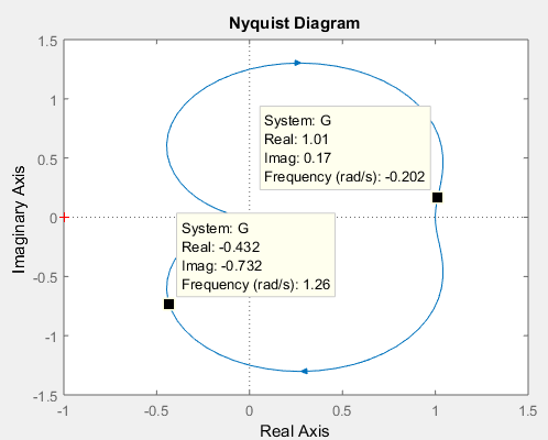
En la parte real se vuelve negativa. En , el diagrama de Nyquist cruza el eje real negativo ya que el término imaginario va a cero. El valor real en el cruce del eje, punto Q^’ en la Figura 4 (c), es -0.874. Continuando hacia, la parte real es negativa, y la parte imaginaria es positiva. A frecuencia infinita:

o cero a los 90°. aproximadamente.

Alrededor del semicírculo infinito desde el punto C hasta el punto D que se muestra en la Figura 4(b), los vectores giran en sentido horario, cada uno 180°. Por lo tanto, la resultante sufre una rotación en sentido antihorario de 3×180, comenzando en el punto C’ y terminando en el punto D’ de la Figura 4 (c).

Diagrama de Nyquist con Matlab

Considere la siguiente función de transferencia a lazo abierto:

Para elaborar el Diagrama de Nyquist, podemos utilizar los siguientes comandos en el command window de Matlab:

>> s=tf(‘s’)

>> G=1/(s^2+0.8*s+1)

>> nyquist(G)

Esta línea de comandos genera la siguiente gráfica:

Podemos obtener información sobre puntos de interés en el diagrama de Nyquist haciendo clik una vez sobre el punto de interés en el contorno:

Siguiente:

Fuentes:

1. Modern_Control_Engineering, Ogata 4t
2. Control Systems Engineering, Nise
3. Sistemas de Control Automatico, Kuo

Revisión literaria hecha por:

Prof. Larry Francis Obando – Technical Specialist – Educational Content Writer

Se hacen trabajos, se resuelven ejercicios!!

WhatsApp:  +34633129287  Atención Inmediata!!

Twitter: @dademuch

Copywriting, Content Marketing, Tesis, Monografías, Paper Académicos, White Papers (Español – Inglés)

Escuela de Ingeniería Electrónica de la Universidad Simón Bolívar, USB Valle de Sartenejas.

Escuela de Ingeniería Eléctrica de la Universidad Central de Venezuela, UCV CCs

Escuela de Turismo de la Universidad Simón Bolívar, Núcleo Litoral.

Contacto: España. +34633129287

Caracas, Quito, Guayaquil, Cuenca. 

WhatsApp:  +34633129287   +593998524011  

Twitter: @dademuch

FACEBOOK: DademuchConnection

email: dademuchconnection@gmail.com

Sketching the Nyquist Diagram

The Nyquist diagram is also known as «The Polar Trace» of a transfer function G(jω), is a graph of the magnitude of G(jω) against the phase angle of G(jω) in polar coordinates, according to ω variables of zero to infinity. Therefore, The Nyquist diagram is the geometric place of vectors:

conforming ω modified from zero to infinity. Note that, in polar graphs, the phase angles are positive (negative) if they are measured counterclockwise (clockwise) from the positive real axis.

The following Figure shows an example of a Nyquist Diagram:

All points of the polar trace of G(jω) represent the end point of a vector at a given value of ω. The projections of G(jω) on the real and imaginary axes are their real and imaginary components. The magnitude and phase angle of G(jω) must be calculated directly for each frequency ω in order to construct polar traces.

Conceptually, the Nyquist diagram is plotted by substituting the points
of the contour that encloses the right half-plane into the function G(s)H(s).  This process is called mapping. Next Figure shows the process of mapping:

Consider the closed-loop control system of Figure 1:

Figure 1

Thus, in the Nyquist diagram, the contour that encloses the right half-plane, shown in Figure 2, can be mapped through the function G(s)H(s), derived from Figure 1,  by substituting points along the contour into G(s)H(s):

Figure 2

If a contour, A, that encircles the entire right half-plane of the root-locus of the system determined by the characteristic equation 1+ G(s)H(s), is mapped through G(s)H(s), then the number of closed-loop poles, Z, in the right half-plane equals the number of open-loop poles, P, that are in the right half-plane minus the number of counterclockwise revolutions, N, around -1+j0 of the mapping; that is, Z:

Thus, Z must be equal to zero to reach stability.

This mapping is called the Nyquist diagram, or Nyquist plot, of G(s)H(s). For more information an examples, see: The Nyquist Criteria

 

Example

Consider the control system whose block diagram and diagram are shown in the following Figure 3:

Figure 3

Conceptually, the Nyquist diagram is plotted by substituting the points of the contour shown in Figure 4(a) into G(s)H(s):

Each Pole and Zero term of G(s) shown in Figure 3(b) is a vector in Figure 4(a) and 4(b). The resultant vector, B´, found at any point along the contour is in general the product of the Zero vectors divided by the product of the Pole vectors (see Figure 4(c)). Thus, the magnitude of the resultant is the product of the Zero lengths divided by the product of the Pole lengths, and the angle of the resultant is the sum of the Zero angles minus the sum of the Pole angles.

Figure 4

The mapping from point A to point C can also be explained analytically. From
A to C the collection of points along the contour is imaginary. Hence, from A to C,
G(s)H(s)=G(s)*1=G(s)=G(jω), or from Figure 3(b):

At zero frequency:

Thus, the Nyquist diagram starts at 50/3 at an angle of 0^°. As ω increases the real part remains positive, and the imaginary part remains negative.

At  the real part becomes negative. At , the Nyquist diagram crosses the negative real axis since the imaginary term goes to zero. The real value at the axis crossing, point Q^’ in Figure 4(c), is -0.874. Continuing toward , the real part is negative, and the imaginary part is positive. At infinite frequency:

or approximately zero at 90°.

Around the infinite semicircle from point C to point D shown in Figure 4(b), the vectors rotate clockwise, each by 180°. Hence, the resultant undergoes a counterclockwise rotation of 3×180, starting at point C’ and ending at point D’ of Figure 4(c).

Nyquist diagram with Matlab

Consider the following open loop transfer function:

To create the Nyquist Diagram of the system, use the following commands in the command window of Matlab:

>> s=tf(‘s’)

>> G=1/(s^2+0.8*s+1)

>> nyquist(G)

This line of commands yields:

We can obtain information of points of interest in the Nyquist Diagram by cliking once over the contour. This yields:

Sources:

1. Modern_Control_Engineering, Ogata 4t
2. Control Systems Engineering, Nise
3. Sistemas de Control Automatico, Kuo

Literature review by:

Prof. Larry Francis Obando – Technical Specialist – Educational Content Writer

I solve problems!!

WhatsApp:  +34633129287  Immediate Attention!!

Twitter: @dademuch

Copywriting, Content Marketing, Tesis, Monografías, Paper Académicos, White Papers (Español – Inglés)

Escuela de Ingeniería Electrónica de la Universidad Simón Bolívar, USB Valle de Sartenejas.

Escuela de Ingeniería Eléctrica de la Universidad Central de Venezuela, UCV CCs

Escuela de Turismo de la Universidad Simón Bolívar, Núcleo Litoral.

Contacto: España. +34633129287

Caracas, Quito, Guayaquil, Cuenca. 

WhatsApp:  +34633129287

Twitter: @dademuch

FACEBOOK: DademuchConnection

email: dademuchconnection@gmail.com

 

 

 

Converting a Transfer Function to State Space representation

To convert a transfer function into state equations in phase variable form, we first convert the transfer function to a differential equation by cross-multiplying and taking the inverse Laplace transform, assuming zero initial conditions. Then we represent the differential equation in state space in phase variable form. An example illustrates the process.

Example 1

Find the state-space representation in phase-variable form for the transfer function shown in Figure (1):

Figure 1

Step 1. Find the associated differential equation:

Cross-multiplying yields:

The corresponding differential equation is found by taking the inverse Laplace  Transform, assuming zero initial conditions:

Step 2. Select the state variables. Choosing the state variables as successive derivatives, we get:

Using this notation, we can rewrite equation (1) as:

Step 3. Differentiating both sides of the last equations, we must find _x1 and _x2, then we use Eq. (2) to find x3. Proceeding in this way we obtain the state equations. Since the output is c=x1, the combined state and output equations are:

Step 4. Expressing the last equations in vector-matrix form, we get the state-space representation of the system as:

At this point, we can create an equivalent block diagram of the systemof Figure 1(a) to help visualize the state variables.We draw three integral blocks as shown in Figure 1(b) and label each output as one of the state variables, xi(t), as shown.

A transfer function with a polynomial in s in the numerator

The transfer function of the previous Example has a constant term in the numerator. If a transfer function has a polynomial in s in the numerator that is of order less than the polynomial in the denominator, as shown in Figure 2(a), the numerator and denominator can be handled separately. First separate the transfer function into two cascaded transfer functions, as shown in Figure 2(b); the first is the denominator, and the second is just the numerator. The first transfer function with just the denominator is converted to the phase-variable representation in state space as demonstrated in the last example. Hence, phase variable x1 is the output, and the rest of the phase variables are the internal variables of the first block, as shown in Figure 2(b).

Figure 2

The second transfer function with just the numerator yields:

Where, after taking the inverse Laplace transform with zero initial conditions, we obtain:

But the derivative terms are the definitions of the phase variables obtained in the
first block. Thus, writing the terms in reverse order to conform to an output equation, we obtain:

Hence, the second block simply forms a specified linear combination of the state
variables developed in the first block.

From another perspective, the denominator of the transfer function yields the
state equations, while the numerator yields the output equation. The next example
demonstrates the process.

Example 2

Find the state-space representation of the transfer function shown in
Figure 3(a).

Step 1. Separate the system into two cascaded blocks, as shown inFigure 3(b).The
first block contains the denominator and the second block contains the numerator.

Step 2. Find the state equations for the block containing the denominator. We notice that the first block’s numerator is 1/24 that of Example 1. Thus, the state equations are the same except that this system’s input matrix is 1/24 that of Example 1.

Step 3. Introduce the effect of the block with the numerator. The second block of
Figure 3(b) yields:

Taking the inverse Laplace transform with zero initial conditions, we get:

But:

Hence:

Thus, the last box of Figure 3(b) ‘‘collects’’ the states and generates the output equation:

Although the second block of Figure 3(b) shows differentiation, this block was implemented without differentiation because of the partitioning that was applied to the transfer function. The last block simply collected derivatives that were already formed by the first block.

Thus, the full state-space representation of the system is:

Once again we can produce an equivalent block diagram that vividly represents
our state-space model:

Sources:

1. Modern_Control_Engineering, Ogata 4t
2. Control Systems Engineering, Nise
3. Sistemas de Control Automatico, Kuo

Literature review by:

Prof. Larry Francis Obando – Technical Specialist – Educational Content Writer

I solve problems!!

WhatsApp:  +34633129287  Immediate Attention!!

Twitter: @dademuch

Copywriting, Content Marketing, Tesis, Monografías, Paper Académicos, White Papers (Español – Inglés)

Escuela de Ingeniería Electrónica de la Universidad Simón Bolívar, USB Valle de Sartenejas.

Escuela de Ingeniería Eléctrica de la Universidad Central de Venezuela, UCV CCs

Escuela de Turismo de la Universidad Simón Bolívar, Núcleo Litoral.

Contacto: España. +34633129287

Caracas, Quito, Guayaquil, Jaén. 

WhatsApp:  +34633129287   

Twitter: @dademuch

FACEBOOK: DademuchConnection

email: dademuchconnection@gmail.com