Block Diagram – Solved problems – Catalog 8 – Mass-spring-damper system and electrical system

In this PDF file, the Block Diagram and the Transfer Function are determined by applying block algebra, from the exercises that are part of control systems, signals and systems, analysis of electrical networks, etc. Each problem has a cost of 12.5 euros. The complete workshop costs 27.5 euros. Payment through Paypal is facilitated.

1. Obtain the transfer function G_(s)=Y_(s)/R_(s) of Figure 1, by two methods: using block algebra reduction techniques and using Mason’s formula.

2. Obtain the transfer function G_(s)=C_(s)/R_(s) of Figure 2, by two methods: using block algebra reduction techniques and using Mason’s formula.

3. Obtain the transfer function G_(s)=C_(s)/R_(s) of Figure 3, by using block algebra reduction techniques .

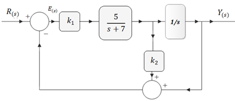
4. Obtain the transfer function G_(s)=Y_(s)/R_(s) of the next Figure, by using block algebra reduction techniques . .  

5. Find the equations of the system in Figure 7 and represent it using state variables. From there determine the block diagram of the system. Then, using block diagram algebra, find the transfer function X_(s)/U_(s). Consider x_(t) as the output and u_(t) as the input. Check the result using Laplace transform.

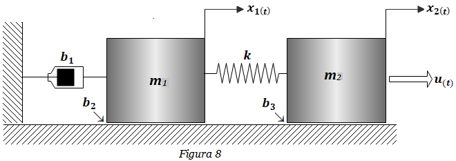
6. Find the equations of the system in Figure 8. Find the matrix representation of the system (state variables). Consider x_1(t) as the output, and u_(t) as the input. Construct the block diagram of the system and use block algebra to determine the transfer function  X_1(s)/U_(s).

7. Find the equations of the system in Figure 22. Determine the transfer function X_1(s)/U_(s). Determine the block diagram of the system from the transfer function obtained.

8. Find the equations of the System in Figure 24. Find the state space representation of the system, considering Θ_1(t) as the output and T_(t) as the input. Find the block diagram of the system and from there, using block algebra, determine the transfer function Θ_1(s)/T_(s).

9. Find the equations of the system in Figure 25. Determine the transfer function X_1(s)/F_(s). Obtain the block diagram of the system from the transfer function obtained (Explain step by step). Graph the response of the system to a step function input using Matlab. Consider k₁= k₂= k₃= 1 N/m, b₁= b₂= b₃=1 N-s/m, m₁= m₂= m₃=1 Kg.

Response graph to the unit step of exercise 9.

10. Determine the differential equations that represent the model of the system in Figure 75. Use the node analysis method. Find the transfer function V_o(s)/V_(s). Make the representation of the system in block diagram from the transfer function V_o(s)/V_(s). Consider R₁=1Ω,  R₂= R₃=1 Ω, L=1 H, C₁=C₂=1 pF.

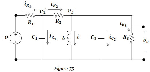
11. Obtain the transfer function V_o(s)/V_(s) of the electrical system in figure 75, from the block diagram of the system obtained in problem 10, using block algebra. Simulate and analyze in Matlab the response of the system to a unit step input

12. Find the state space representation of the System shown in Figure 39 assuming that Θ_4(t) is the output and T_(t) is the input. Draw the block diagram of the system and find the transfer function Θ_4(t)/T_(t). Consider k=2 N-m/rad, b=16 N-m-s/rad, J=4  Kg-m²

13. Find the transfer function Θ_L(s)/E_i(s) of the system shown in Figure 56. Find the state space representation of the system, assuming that Θ_L(t) is the output and that e_i(t) is the input . Represent the System by means of a block diagram. From the block diagram of the system, determine again and by means of block algebra the transfer function Θ_L(s)/E_i(s).

14. Find the transfer function Θ_L(s)/Θ_r(s) of the system shown in Figure 59. Design the block diagram of the system.

15. Find the transfer function Q_2(s)/Q_1(s) of the Liquid Level System shown in Figure 68. Find the state space representation of the System taking q_2(t) as the output, and q_1(t) as the input. Obtain the block diagram of the system and determine the same transfer function using block algebra.

16. A very simplified model of the dynamics of a rocket is shown in Figure 1. A uniform bar of mass m and length 2L, subjected to the force of gravity G (center of gravity of the bar) and to two external forces applied at its lower end: a vertical V_(t) and a horizontal H_(t). It is requested: i) Draw the input and output variables diagram. Characterize the equilibrium point determined by x₍₀₎=0, y₍₀₎=0. Ii) Obtain the system of equations linearized around the equilibrium point. iii) Draw the block diagram of the system. iV) Obtain the transfer functions from it

17. Determine the expression for the output C_(s) of the system of Figure 90

Figure 90

ATTENTION: If you cannot find what you are looking for… .I can solve exercises and block diagram problems for you right away. Please send a message to my WhatsApp and I will give you the solution as soon as possible… +34633129287… you can pay with Paypal and TC

To solve this guide the following rules will be used:

Puedes consultar también:

• Dinámica de un Sistema Masa-Resorte-Amortiguador
• Simulación en Matlab de respuesta en el tiempo de sistema masa-resorte-amortiguador
• Ejercicio de dinámica masa-resorte-amortiguado, función de transferencia.
• Ejercicio de dinámica, variable de estado, función de transferencia. 
• Ejercicio de diagrama de bloques a partir de la Transformada de Laplace
• Ejercicio de Diagrama de bloques a partir de representación en variables de estado 
• Ejercicio de Función de Transferencia a partir de representación en Variables de Estado
• Ejemplo 1 – Función Transferencia de Sistema masa-resorte-amortiguador
• Ejemplo 2 – Función Transferencia de sistema masa-resorte-amortiguador
• Ejemplo 1 – Representación en Variables de Estado de un Sistema Masa-Resorte-Amortiguador
• Función de Transferencia de Sistema Mecánico Rotacional – Ejemplo 1
• Respuesta Transitoria de sistema masa-resorte-amortiguador
• Sistema masa-resorte-amortiguador. Problemas resueltos. Catálogo 1. 
• Sistema masa-resorte-amortiguador. Problemas resueltos. Catálogo 2.
• Sistema masa-resorte-amortiguador. Problemas resueltos. Catálogo 3.
• Sistema masa-resorte-amortiguador con engranajes. Problemas resueltos. Catálogo 4.
• Función de transferencia de sistema eléctrico – Problemas resueltos – Catálogo 5
• Motor DC – Problemas resueltos de sistema electromecánico – Función de Transferencia – Catálogo 6
• Función de transferencia de sistema electrónico – Problemas resueltos – Catálogo 7
• Análisis de respuesta transitoria – Problemas resueltos – Catálogo 9
• Error en estado estable estable – problemas resueltos – catálogo 10
• Convolución – Problemas resueltos – Catálogo 11

Made by Prof. Larry Francis Obando – Technical Specialist – Educational Content Writer – Twitter: @dademuch

Mentoring Académico / Emprendedores / Empresarial

Copywriting, Content Marketing, Tesis, Monografías, Paper Académicos, White Papers (Español – Inglés)

Escuela de Ingeniería Electrónica de la Universidad Simón Bolívar, USB Valle de Sartenejas.

Escuela de Ingeniería Eléctrica de la Universidad Central de Venezuela, UCV CCs

Escuela de Turismo de la Universidad Simón Bolívar, Núcleo Litoral.

Contacto: Jaén – España: Tlf. 633129287

Caracas, Valladolid, Quito, Guayaquil, Jaén, Villa Franca de Ordizia.

WhatsApp: +34 633129287

Twitter: @dademuch

FACEBOO DademuchConnection

email: dademuchconnection@gmail.com